Manipulate and Visualize Raster data with leaflet and tmap in R

What is Raster Data?

Raster or “gridded” data are data that are stored in pixels. In the spatial world, each pixel represents an area on the Earth’s surface. In this post will focus raster package and its key function for importing and manipulating raster objects. I expect that toward the end of the post, you will have a glimpse of this package and you will be able to:

describe what a raster dataset is and its fundamental attributes.
Import rasters into R using the raster library.
Visualize raster interactive and with static map
Perform raster calculations in R.

Loading a raster file

To work with rasters in R, we need two key packages, sp and raster [@raster]. To install the raster package you can use install.packages('raster'). When you install the raster package, sp should also install. Also install the rgdal package install.packages('rgdal'). Among other things, rgdal will allow us to export rasters to GeoTIFF format. Once installed, we load the package in our session using the require function and start working with raster data.

require(leaflet)
require(raster)

The raster package can read raster files in several formats, including some ‘natively’ supported formats and other formats via the rgdal package. Supported formats for reading include GeoTiff, ESRI, ENVI, and ERDAS. raster package also read data stored in Unidata netCDF format. Here is an example of reading the netCDF file and import the sea surface temperature in our session for further processing and visualization.

sst = raster("./modis_sst_monthly_climatological/sst_climatology_Feb_4km_modis.nc", varname = "sst4")

Next, let’s look at the attributes of the raster dataset we just loaded in our session.

sst

class      : RasterLayer 
dimensions : 4320, 8640, 37324800  (nrow, ncol, ncell)
resolution : 0.04166667, 0.04166667  (x, y)
extent     : -180, 180, -90.00001, 90  (xmin, xmax, ymin, ymax)
crs        : +proj=longlat +datum=WGS84 +no_defs 
source     : e:/MatlabWorking/modis_sst_monthly_climatological/sst_climatology_Feb_4km_modis.nc 
names      : X4um.Sea.Surface.Temperature 
zvar       : sst4

Notice key attributes about this raster.

dimensions—the “size” of the file in pixels
nrow, ncol— the number of rows and columns in the data (imagine a spreadsheet or a matrix).
ncells—the total number of pixels or cells that make up the raster.
resolution—the size of each pixel (in meters in this case). 1 meter pixels means that each pixel represents a 1m x 1m area on the earth’s surface.
extent—the spatial extent of the raster. This value will be in the same coordinate units as the coordinate reference system of the raster.
coord ref—the coordinate reference system string for the raster. This raster is in UTM (Universal Trans Mercator) zone 11 with a datum of WGS 84

Work with Rasters in R

Now that we have the raster loaded into R, let’s grab some key raster attributes.

Define Min/Max Values

By default this raster doesn’t have the min or max values associated with it’s attributes Let’s change that by using the setMinMax() function. In short, the function calculates and save the min and max values of the raster to the raster object

sst %>% setMinMax()

class      : RasterLayer 
dimensions : 4320, 8640, 37324800  (nrow, ncol, ncell)
resolution : 0.04166667, 0.04166667  (x, y)
extent     : -180, 180, -90.00001, 90  (xmin, xmax, ymin, ymax)
crs        : +proj=longlat +datum=WGS84 +no_defs 
source     : e:/MatlabWorking/modis_sst_monthly_climatological/sst_climatology_Feb_4km_modis.nc 
names      : X4um.Sea.Surface.Temperature 
values     : -1.86, 32.145  (min, max)
zvar       : sst4

Notice the minimum and maximum values of sea surface temperature is now included as attributes and shows the min and max values for the pixels in the raster. We can further view the raster’s min, max, range, median, mean, sd values and the range of values contained within the pixels.

cellStats(x = sst, stat = min);

[1] -1.86

cellStats(x = sst, stat = max);

[1] 32.145

cellStats(x = sst, stat = range);

[1] -1.860 32.145

cellStats(x = sst, stat = mean);

[1] 16.6292

cellStats(x = sst, stat = median);

[1] 19.5

cellStats(x = sst, stat = sd)

[1] 10.16192

View CRS

First, let’s consider the Coordinate Reference System (CRS).

sst %>% crs()

CRS arguments: +proj=longlat +datum=WGS84 +no_defs

We then check for its geographical extent

sst %>% extent()

class      : Extent 
xmin       : -180 
xmax       : 180 
ymin       : -90.00001 
ymax       : 90

Raster Pixel Values

We can also create a histogram to view the distribution of values in our raster. Note that the max number of pixels that R will plot by default is 100,000. We can tell it to plot more using the maxpixels attribute. Be careful with this, if your raster is large this can take a long time or crash your program.

Since our raster is a surface temperature of the ocean, we know that each pixel contains temperature values measured in degree Celsius about our area of interest.

sst %>% 
  values() %>% 
  hist(main="Distribution of temperature values", 
     col= "maroon")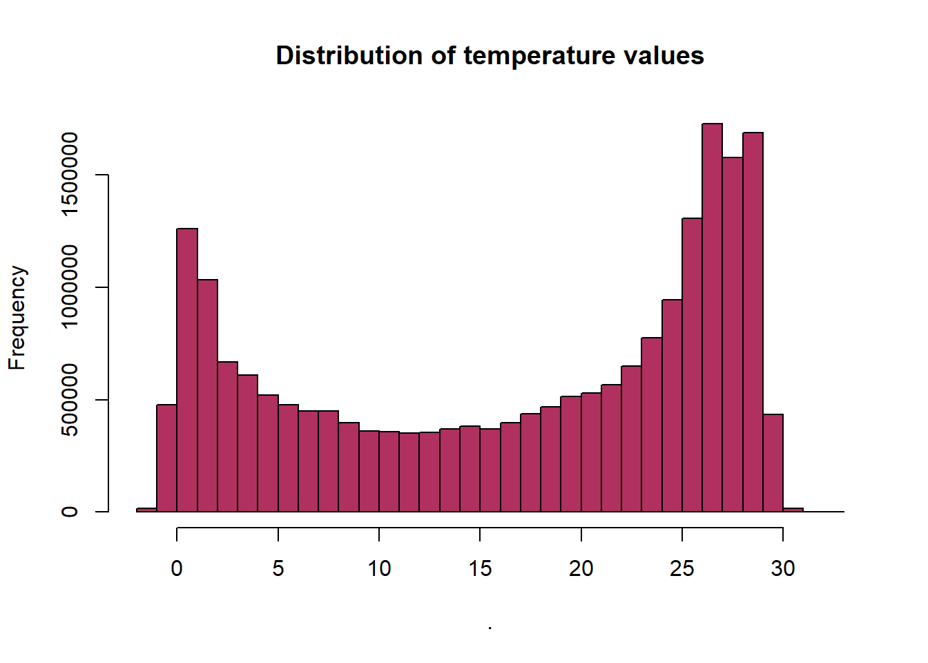

This is an easy and quick data checking tool. Are there any totally weird values?

Crop raster

We notice that the dataset cover the global extent, hence we need to crop it to small areas of interest. We can crop rasters in R using various method, however, in this case,I chose a manual work of defining a geographical, which span from longitude 38 and 60 East and latitude 6 and 0 South of the equator. We define the bounding box of the area of interest using the extent function. This is how we’d crop using a GIS shapefile (with a rectangular shape)

tz.bbox = extent(38, 60, -6, 0)

Once we have defined the geographical extent of the area of interest, we can parse it into a crop function as an argument to chop sea surface temperature only the area of interest

sst.tz = sst %>% raster::crop(tz.bbox)

sst.tz %>% setMinMax()

class      : RasterLayer 
dimensions : 144, 528, 76032  (nrow, ncol, ncell)
resolution : 0.04166667, 0.04166667  (x, y)
extent     : 38, 60, -6.000008, -7.629395e-06  (xmin, xmax, ymin, ymax)
crs        : +proj=longlat +datum=WGS84 +no_defs 
source     : memory
names      : X4um.Sea.Surface.Temperature 
values     : 22.15, 29.965  (min, max)

sst.tz[sst.tz < 26 | sst.tz > 29] = NA

Map the raster interactive

Finally, we will plot the sea surface temperature within the area of interest on a leaflet interactive map. The leaflet::addRasterImage()function allows the user to plot raster objects on the map. The leaflet::addCircles() function allows the user to plot point data on the map. For a more detailed example, click this link.

In order to render the RasterLayer as an image, each cell value must be converted to an RGB(A) color. I used the colorNumeric function to specify the color scale as the chunk below highlight:

pal = colorNumeric(c("#7f007f", "#0000ff",  "#007fff", "#00ffff", "#00bf00", "#7fdf00",
"#ffff00", "#ff7f00", "#ff3f00", "#ff0000", "#bf0000"), values(sst.tz),  na.color = "transparent")

sst.color = c("#7f007f", "#0000ff",  "#007fff", "#00ffff", "#00bf00", "#7fdf00",
"#ffff00", "#ff7f00", "#ff3f00", "#ff0000", "#bf0000")

leaflet() %>% 
  addTiles() %>%
  addRasterImage(x = sst.tz , 
                 colors = pal, 
                 opacity = 1) %>%
  addLegend(pal = pal, values = values(sst.tz),
    title = "Temperature")

We can also map with ggplot2 package [@ggplot]

require(ggplot2)
aoi = spData::world %>% 
  sf::st_crop(xmin = 38, xmax = 60, ymin = -6, ymax = 0)

sst.tz %>%
  as.data.frame(xy = TRUE) %>%
  dplyr::rename(z = 3) %>%
  ggplot(aes(x = x, y = y, fill = z)) + 
  geom_raster()+
  scale_fill_gradientn(colours = sst.color, breaks = seq(26,30,0.5), guide = guide_colorbar(title.position = "right", title = expression(Temperature~(degree*C)), title.theme = element_text(angle = 90)))+
  ggspatial::layer_spatial(data = aoi)+
  coord_sf(xlim = c(39,58), ylim = c(-5.6,-0.5))+
  theme_bw() +
  theme(axis.title = element_blank())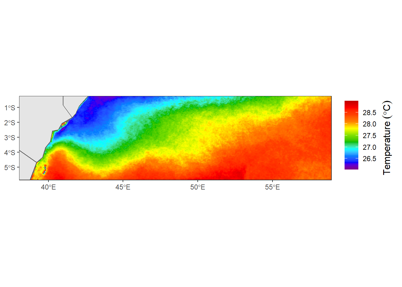

For greater control in plotting the raster, you might want to use the tmap package.

library(tmap)

tm_shape(sst.tz) + 
  tm_raster(style= "sd", n = 10 , palette = "Greys")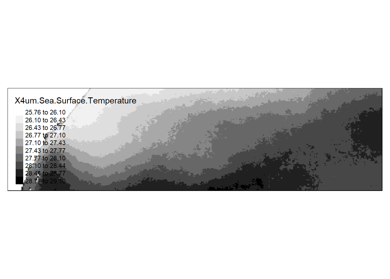

The style parameter controls the classification method (standard deviation is chosen here). Other options include pretty, jenks and kmeans just to name a few. If you want to adopt a continuous color scheme, set style to cont. We’ll also move the legend box off to the side.

tm_shape(sst.tz) + 
  tm_raster(style= "cont", n = 10 , palette = "Greys", title = "surface\nTemperature\n(degree)")+ 
  tm_legend(outside = TRUE)

We can use st_crop function from sf package to chop any shapefile to the area of interest. For this case, I will first pull the world polygon shapefile from spData package and then chop the geographical extent that matches those used to chop the sea surface temperature above [@spdata].

aoi = spData::world %>% 
  sf::st_crop(xmin = 38, xmax = 60, ymin = -6, ymax = 0)

Once we have shapefile of the area of interest, we can overlay this vector layer into sea surface temperature.

tm_shape(shp = sst.tz) + 
  tm_raster(style= "cont", n = 10 , palette = "Greys", title = "surface\nTemperature\n(degree)")+
  tm_shape(shp = aoi) + 
  tm_borders() + 
  tm_legend(outside = TRUE)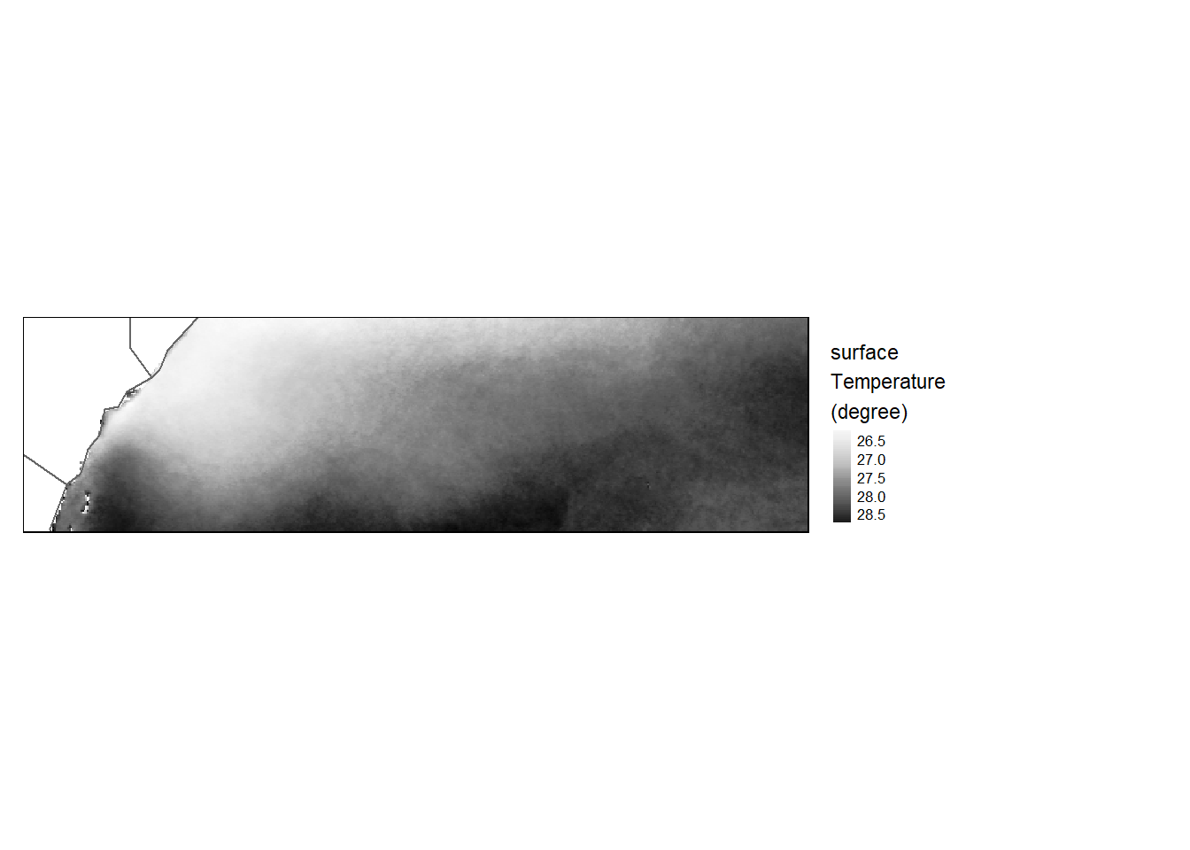

Decreasing pixel resolution

To decrease a raster’s resolution, use the aggregate function to resample the raster. Here, we’ll resample by a factor of 20 (i.e. 20x20 pixels will be aggregated to a single cell) and use the arithmetic mean to compute the cell’s output value.

sst_downsample = aggregate(sst.tz, 
                            fact=20, 
                            fun=mean, 
                            expand=TRUE)

tm_shape(sst_downsample) +
  tm_raster(style= "cont", title = "surface\nTemperature\n(degree)") +
  tm_shape(shp = aoi) + 
  tm_borders() + 
  tm_legend(outside = TRUE)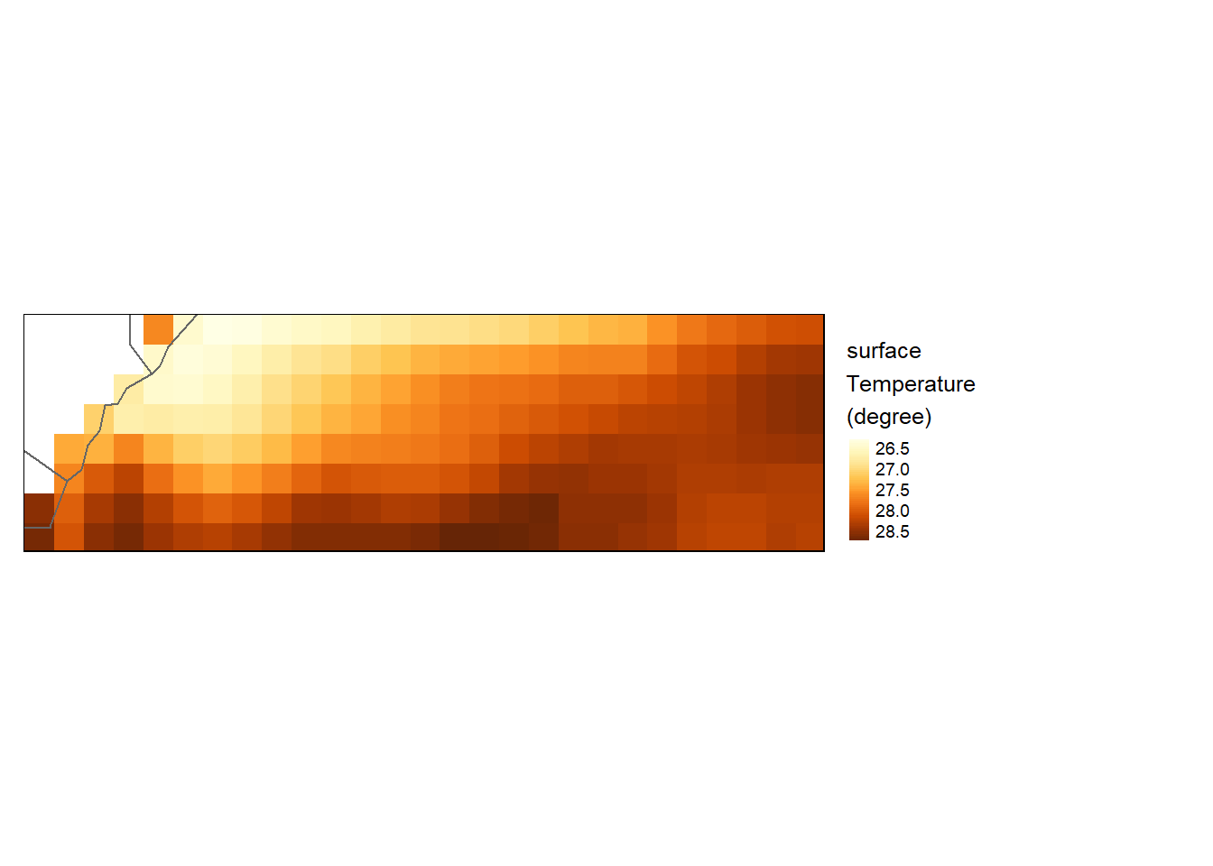

Increasing pixel resolution

To increase a raster’s resolution, we’ll use the disaggregate function. Here we’ll double the pixel resolution (fact=2).

sst_upsample = disaggregate(sst.tz, fact = 2)

tm_shape(sst_upsample) +
  tm_raster(style= "cont", title = "surface\nTemperature\n(degree)") +
  tm_shape(shp = aoi) + 
  tm_borders() + 
  tm_legend(outside = TRUE)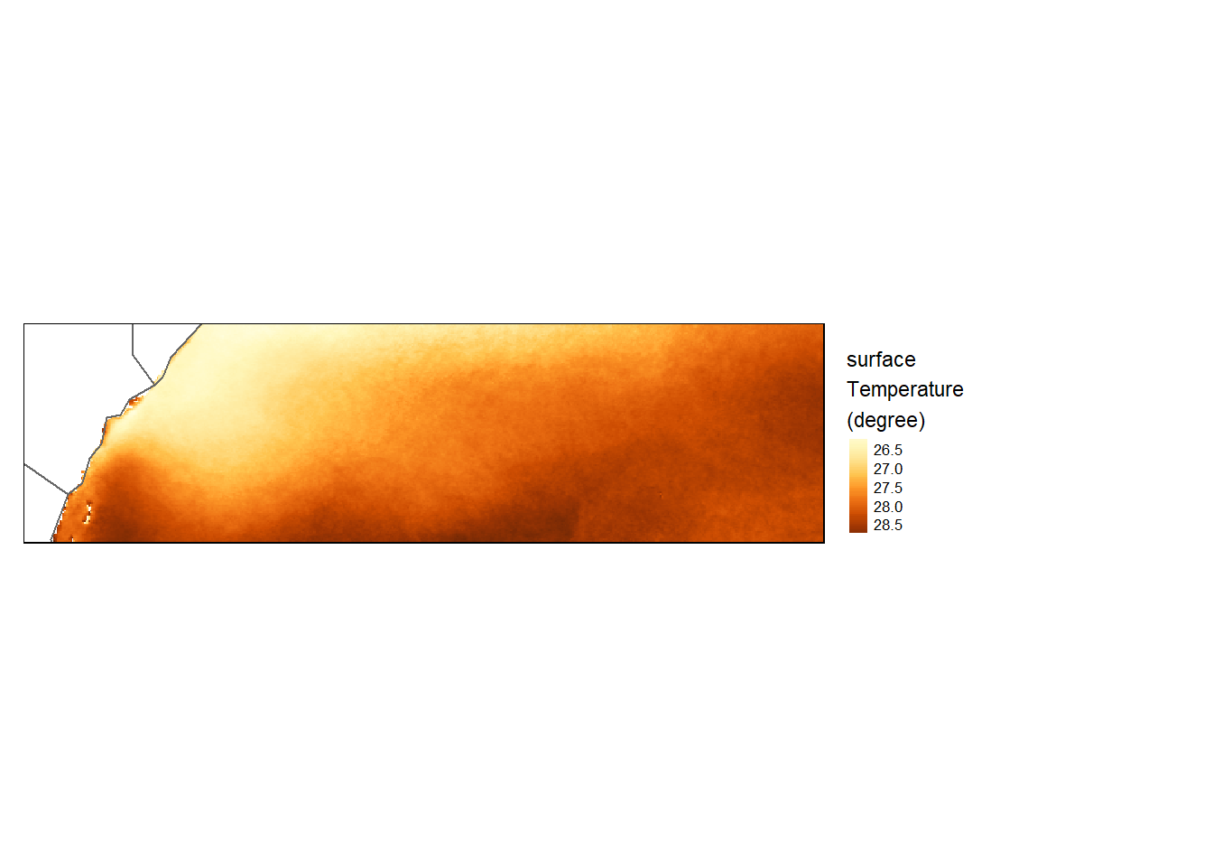

Map algebra

Local operations

Unary operations

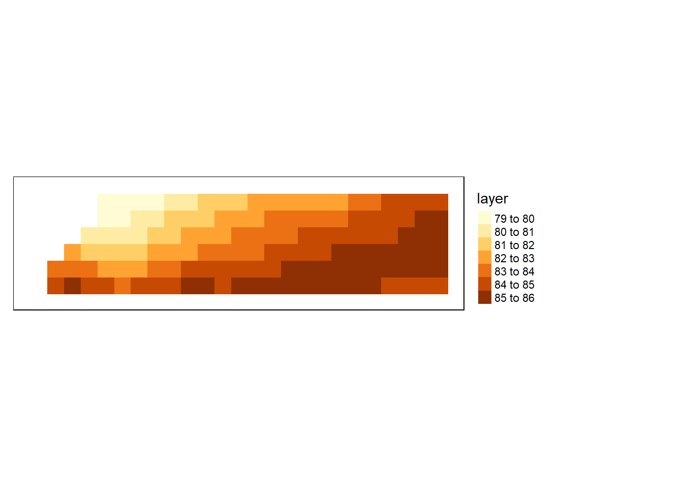
Here we convert temperature from degree to fahrenheit using a degree2fahrenheit function from wior package [@wior].

sst.far = sst_downsample %>% 
  wior::degree2fahrenheit()

tm_shape(sst.far) +
  tm_raster(style= "cont", title = "surface\nTemperature\n(Fahrenheit)") +
  tm_shape(shp = aoi) + 
  tm_borders() + 
  tm_legend(outside = TRUE)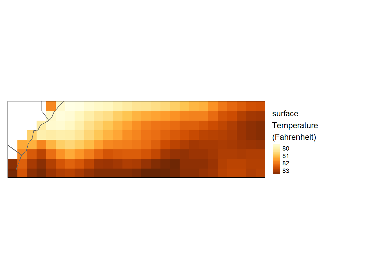

Binary operation

Next, we’ll use conditional statements to create two intermediate rasters, then combine them using the Boolean operator I to identify all pixels whose elevation value is greater than 27.50 and less than 28.25 degree celcius

sst.bin = sst_downsample > 27.5 & sst_downsample < 28.25

tm_shape(sst.bin) +
  tm_raster(style= "cont", title = "surface\nTemperature\n(Fahrenheit)") +
  tm_shape(shp = aoi) + 
  tm_borders() + 
  tm_legend(outside = TRUE)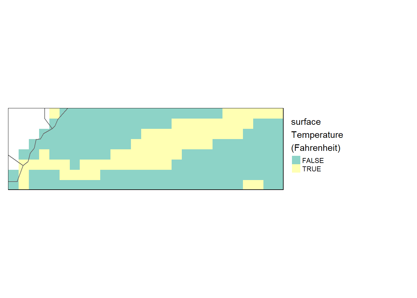

Focal Operations

Focal operations require that a kernel be defined. The kernel can be defined via a weighted matrix (as used in the following example) or a function. The kernel definition is passed to the w parameter in the focal function.

sst_focal = focal(sst_downsample, w=matrix(1/3,nrow=3,ncol=3))

tm_shape(sst_focal) + tm_raster() + tm_legend(outside = TRUE)