Text mining in R

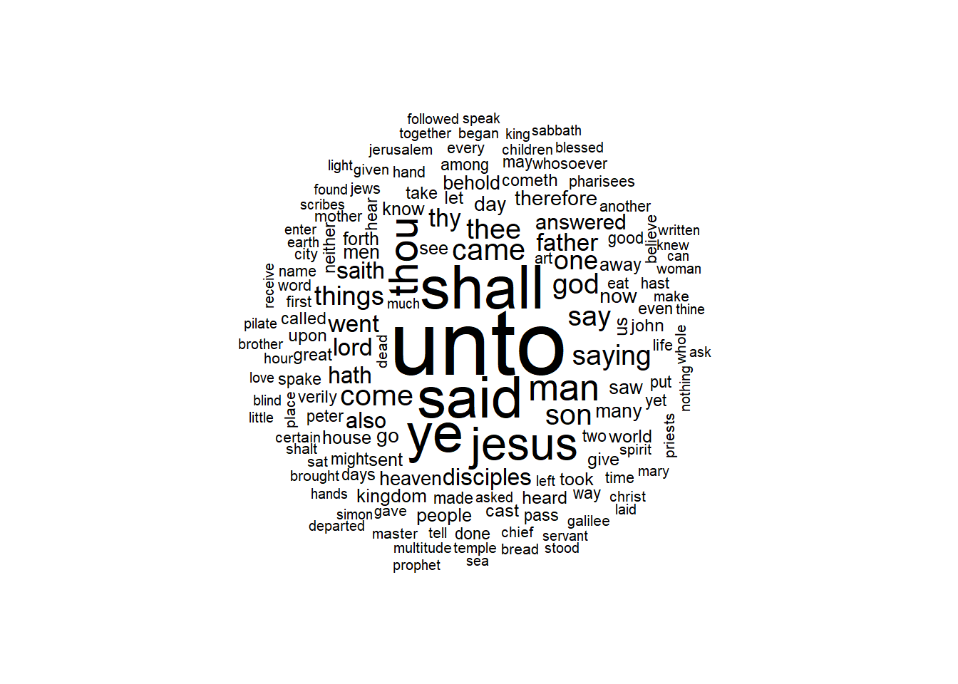
Most common positive and negative words

There are a variety of methods and dictionaries that exist for evaluating the opinion or emotion in text. The tidytext package contains several sentiment lexicons. Three general-purpose lexicons are afinn, bing and nrc. These three lexicons are based on unigrams—single words. They contain many English words and the words are assigned scores for positive/negative sentiment, and also possibly emotions like joy, anger, sadness, and so forth. The nrc lexicon categorizes words in a binary fashion (“yes”/“no”) into categories of positive, negative, anger, anticipation, disgust, fear, joy, sadness, surprise, and trust. The bing lexicon categorizes words in a binary fashion into positive and negative categories. The AFINN lexicon assigns words with a score that runs between -5 and 5, with negative scores indicating negative sentiment and positive scores indicating positive sentiment. All of this information is tabulated in the sentiments dataset, and tidytext provides a function get_sentiments() to get specific sentiment lexicons without the columns that are not used in that lexicon.

bing = get_sentiments(lexicon = "bing") #c("afinn", "bing", "loughran", "nrc")

With data in a tidy format, sentiment analysis can be done as an inner join. This is another of the great successes of viewing text mining as a tidy data analysis task; much as removing stop words is an antijoin operation, performing sentiment analysis is an inner join operation.

bible.book.sentiments = bible.book.freq %>% 
  inner_join(bing, by = "word")

One advantage of having the data frame with both sentiment and word is that we can analyze word counts that contribute to each sentiment.

bible.book.sentiments  %>%
  filter(n > 20) %>%
  mutate(n = ifelse(sentiment == "negative", -n, n)) %>%
  mutate(word = reorder(word, n)) %>%
  ggplot(aes(x = word, y = n, fill = sentiment)) +
  geom_col(alpha = .8) +
  coord_flip() +
  labs(y = "Contribution to sentiment")+
  theme(panel.background = element_blank(), panel.grid = element_blank(),
        legend.position = c(.75,.25))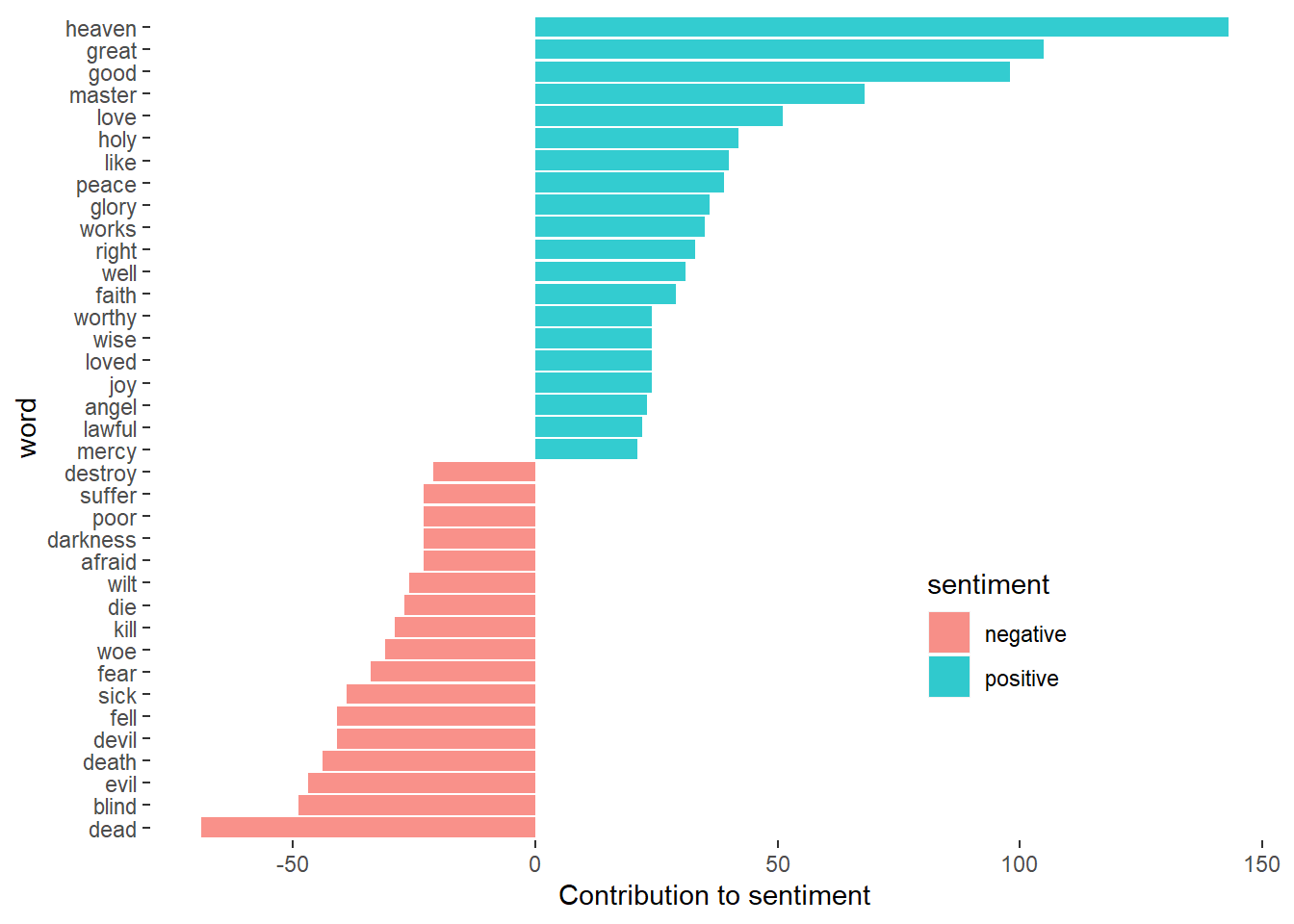

This can be shown visually, and we can pipe straight into ggplot2, if we like, because of the way we are consistently using tools built for handling tidy data frames. For example, consider the wordcloud package, which uses base R graphics. Let’s look at the most common words in four Gospal of the Bible as a whole again, but this time as a wordcloud in Figure 2.5.

bible.book.sentiments %>% 
  with(wordcloud::wordcloud(words = word, freq = n, 
                            max.words =150, random.order = F))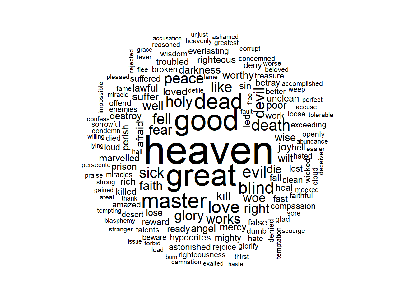

In other functions, such as comparison.cloud(), you may need to structure a data frame the data frame so that the common words column become a rowname column_to rownames() function from dplyr package. Let’s spread the the sentiment to tag positive and negative words as separate variable using spread().

bible.book.sentiments %>% 
  spread(key = sentiment, value = n, fill = 0)  %>% 
  column_to_rownames(var = "word") %>%
  wordcloud::comparison.cloud(colors = c("#F8766D", "#00BFC4"), 
                              max.words = 150, use.r.layout = F, 
                              match.colors = T, random.order = F, title.size = 0.01)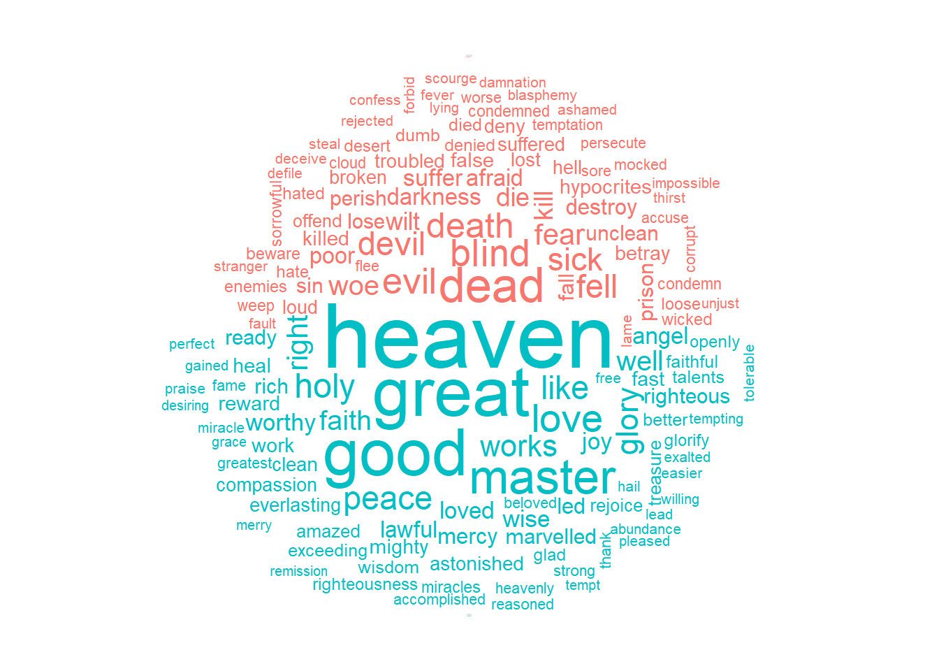

Extracting PDF Text with R and Creating Tidy Data

In the digital age of today, data comes in many forms. Many of the more common file types like CSV, XLSX, and plain text (TXT) are easy to access and manage. Yet, sometimes, the data we need is locked away in a file format that is less accessible such as a PDF. If you have ever found yourself in this dilemma, fret not — pdftools has you covered. In this post, you will learn how to: use pdftools to extract text from a PDF, use the stringr package to manipulate strings of text, and create a tidy data set. In anticipation of March Madness and being a University of Cincinnati alumnus along with some other my other Datazar constituents, I have chosen to extract season statistics from the UC men’s basketball team. In the end, I will create a tibble showing season statistics for minutes played, field goal percentage, total points, and average points per game for each player. The first step is to load the packages that are needed using library(). The stringr package is a member of the tidyverse collection of R packages (more on that here if you are not familiar). The packages in therein are designed to make data science easy. I highly recommend purchasing R for Data Science by Hadley Wickham and Garrett Grolemund. It is a great book for beginners as well as a pocket reference for more advanced programmers. I use this book almost every day — it goes where I go.

The next step is to load your PDF into your Datazar project. I am going to call my new object ‘UC_text’ and I am going to use the pdf_text command to read the text of my file. The read_lines() function reads the lines of our new file.

wiomsa.smp = pdftools::pdf_text("e:/Symposium-ProgrammeFINAL_titles.pdf") %>%
  readr::read_lines()

wiomsa.smp %>% head()

## [1] "                                                    LT 1"                                             
## [2] "                                  Session I: Stock status assessment"                                 
## [3] " 1100    Conand, C.; C. Michel; D. Chamari; F. Stella; G. Rodney; L. Thierry; L. Marc; M. Twalibu; M."
## [4] "         Thierry; S. Stanley; Y. Saleh; F. Kim - Fisheries and management of sea cucumbers in the"    
## [5] "         WIO: an update"                                                                              
## [6] " 1120    Everett, B.; S. Fennessy; N. van den Heever - Tracking temporal and spatial patterns in the"

In the next series of steps, I will use functions in the stringr package to manipulate the lines of text into a desirable form. The first problem to tackle is the whitespace between the different elements in each line of text. The str_squish() function reduces the repeated whitespace between each string. I also need to remove the comma between each player’s first and last name. I’ll use str_replace_all() to remove the comma.

wiomsa.smp %>% 
  str_squish() %>% 
  str_replace_all(pattern = ";", " ") %>% 
  str_replace_all(pattern = "-", "")%>% 
  str_replace_all(pattern = "11th WIOMSA Scientific Symposium", "")%>% 
  str_replace_all(pattern = "WIO", "") %>%  
  as_tibble() %>% 
  rename(text = 1)%>% 
  unnest_tokens(word, text) %>%
  anti_join(get_stopwords(), by = "word") %>%
  group_by(word) %>% count() %>% ungroup() %>% slice(-c(1:115)) %>%
  arrange(desc(n))

## Warning: Calling `as_tibble()` on a vector is discouraged, because the behavior is likely to change in the future. Use `tibble::enframe(name = NULL)` instead.
## This warning is displayed once per session.

## # A tibble: 3,991 x 2
##    word       n
##    <chr>  <int>
##  1 m        290
##  2 s        248
##  3 j        220
##  4 c        165
##  5 l        142
##  6 n        129
##  7 r        128
##  8 t        117
##  9 marine   116
## 10 p         98
## # ... with 3,981 more rows

tabulizer package

Earlier this year, a new package called tabulizer was released in R, which allows you to automatically pull out tables and text from PDFs. Note, this package only works if the PDF’s text is highlightable (if it’s typed) — i.e. it won’t work for scanned-in PDFs, or image files converted to PDFs.

If you don’t have tabulizer installed, just run install.packages(“tabulizer”) to get started. After you have tabulizer installed, we’ll load it, and define a variable referencing an example PDF.

How to scrape tables from a PDF

You can extract tables from this PDF using the extract_tables function. we can add parameters to the function to specify the output flag to be data.frame, and set header = TRUE, to get back a list of data frames corresponding to the tables in the PDF. Once we have the results back, we can refer to any individual PDF table like any data frame we normally would in R.

program.table = tabulizer::extract_tables("e:/Symposium-ProgrammeFINAL_titles.pdf",
                          output = "data.frame", header = TRUE )

How to scrape text from a PDF

Scraping text from our sample PDF can be done using extract_text:

program.text = tabulizer::extract_text("e:/Symposium-ProgrammeFINAL_titles.pdf", )

program.text %>% as_tibble() %>% 
  rename( text = 1) %>% 
  separate(col = text, into = c("authors", "title"), sep = "-") %>% 
  select(title) %>%
  separate_rows(title, sep = "\r\n") %>%
  unnest_tokens(word, text) %>% anti_join(get_stopwords())

program.text %>% 
  str_replace_all(pattern = "\r\n", replacement = " ") %>% 
  as_tibble()%>%
  rename( text = 1) %>%
  # separate_rows(title, sep = "\r\n")