plotting the Spatial distribution of Chlorophyll in Mafia Channel from MODIS

Data

I used the chlorophyll-a dataset from MODIS. You can easily extract and download level 3 chlorophyll and sea surface temperature data of the area of interest from NASA ocean color. Once you have downloaded the dataset and saved them in working directory of your local machine. The data is in the netCDF format as an array of five variables. But we are only interested with three variables describe below;

• longitude; degree east also called eastings
• latitude; degree north also called northings
• chl_oc3; Chlorophyll-a concentration in sea water as measured by the MODIS sensor mapped in grid of longitude and latitude. The cell without chl-a values are assigned a missing value of -32767 and

You simply read this files with the nc_open() function from the ncdf4 package (Pierce 2017)

chl = ncdf4::nc_open("./Chl-a/M2012092-2012121.vw.all_products.MYO.median.01apr12-30apr12.1368530290.data.nc")

Scientist in R community are familiar with ncdf4 package and often use its function to import and extract variables from netCDF files (Pierce 2017). For instance many would read the variables embedded in the file using the ncvar_get() function. However, in this post I switched to oceanmap package because it offers some simple but powerful functions to work high dimension data (Bauer 2019). For example, I used nc2raster() function to convert the ncdf4-object to a Raster object, setting the time variable as layer name. This chunk below shows;

## for display the code only, but never run
chl.dat.raster = chl %>%
    oceanmap::nc2raster(varname = "chl_oc3",
                       t = 1, 
                       lonname="longitude", 
                       latname="latitude", 
                       date=T, layer = 1)

Once we have the raster object, we can check its geographical extent with chl.dat.raster %>% raster::extent() command;

chl.dat.raster %>% raster::extent()

class      : Extent 
xmin       : 38 
xmax       : 42.99595 
ymin       : -12.9955 
ymax       : -2.999101 

We notice that the raster object lies in longitude between 38°E38 and rmetR::LonLabel(43) and latitude 12°S and 3°S. This extent cover the entire coastal area of Tanzania. Because our interest is in Rufiji–Mafia Channel, we need to chop only the cell that fall within this area. I used the extent() function from raster to chop only the area. In order to do this, I first create the extent layer using the maximum and minimum values of longitude and latitude and assign it as rufiji.extent. I used used this extent layer to crop the large raster layer and assign it a name as chl.mafia

## create chopping object
rufiji.extent = raster::extent(39.3, 40.0, -8.0,-7.5)
## chop the raster object
chl.mafia = raster::crop(x = chl.dat.raster, y = rufiji.extent) 

We can have a glimpse of the cropped raster object of Rufiji–Mafia Channel

chl.mafia

class      : RasterLayer 
dimensions : 112, 156, 17472  (nrow, ncol, ncell)
resolution : 0.004492763, 0.004494785  (x, y)
extent     : 39.29841, 39.99928, -8.001797, -7.498381  (xmin, xmax, ymin, ymax)
crs        : +proj=longlat +ellps=WGS84 
source     : memory
names      : X2012043010 
values     : 0.07688248, 30.65916  (min, max)

We notice that the value of chlorophyll-a range from 0.07688248 to 30.65916 mgm^-3. The range is quite big and the maximum value is usual higher in poor coastal water like Rufiji. Based on local knowledge, this channel is one of the most productive marine habitats in the Western Indian Ocean Region, however, its values hardly exceed 3 mgm^-3. Therefore, we need to remove extremely higher values. I used the clamp() function from raster package (Hijmans 2017) to assign values to a minimum and maximum value. That is, all values below the lower clamp value and above the upper clamp value become NA (or the lower/upper value if useValue=TRUE)

##
#chl.mafia[chl.mafia > 3.1] = NaN

chl.mafia = chl.mafia %>% 
  raster::clamp(upper = 3.1, # lower clamp value
                lower = 0.1,  # upper clamp value
                usevalues = FALSE # force value to NA
                )
chl.mafia

class      : RasterLayer 
dimensions : 112, 156, 17472  (nrow, ncol, ncell)
resolution : 0.004492763, 0.004494785  (x, y)
extent     : 39.29841, 39.99928, -8.001797, -7.498381  (xmin, xmax, ymin, ymax)
crs        : +proj=longlat +ellps=WGS84 
source     : memory
names      : X2012043010 
values     : 0.1, 3.1  (min, max)

Mapping chl-a

So far, you’ve learned the tools to get your data into R , transform and format in a convenient structure for analysis. However, visualize this data can help us better understand the spatial distribution of chl-a in this channel. R has several tools that can turn data into plots. But my focus in this post is to map chl-a using oceanmap (Bauer 2019) package and ggplot2 package (Wickham 2016). oceanmap package has v() function that is used to plot 2D oceanographic data. For this case we use this function to map the spatial distribution of chlorophyll-a in the Rufiji–Mafia channel (Figure ??).

oceanmap::v(obj = chl.mafia, cbpos = "b", pal = "jet",
            cb.xlab = expression("Chlorophyll-a (mg m"^-3*")"), bwd = 0.01, grid = F, 
            # Save = T, plotname = "rufiji_mafia_chl", fileformat = "png", width = 10, height = 5, 
            replace.na = F, axeslabels = FALSE)

You can also use ggplot2 package, that use the grammar of graphics, to make lot similar to those made with oceanmap package. For instance, the chunk below shows codes from ggplot used to generate figure 1.

chl.mafia.df = chl.mafia %>% 
  raster::as.data.frame(xy = TRUE) %>% rename(lon = x, lat = y, chl = 3)

ggplot() + 
  geom_raster(data = chl.mafia.df, aes(x = lon,  y = lat, fill = chl))+
  geom_sf(data = bongo, fill = "grey80", col = "black")+
  coord_sf(xlim = c(39.29841, 39.99928), c(-8.001797, -7.498381))+
  scale_fill_gradientn(colours = oce::oce.colorsJet(120), na.value = "white", breaks = seq(0,3.2,0.5))+
  metR::scale_x_longitude(ticks = .2) + 
  metR::scale_y_latitude(breaks = c(-7.92, -7.80, -7.68, -7.56))+
  guides(fill = guide_colorbar(title = expression(Chlorophyll-a~(mg~m^{-3})),
                               title.position = "right",
                               title.theme = element_text(angle = 90), 
                               barwidth = unit(.5, "cm"),barheight = unit(7.5, "cm"),title.hjust = .5))+
  theme_bw()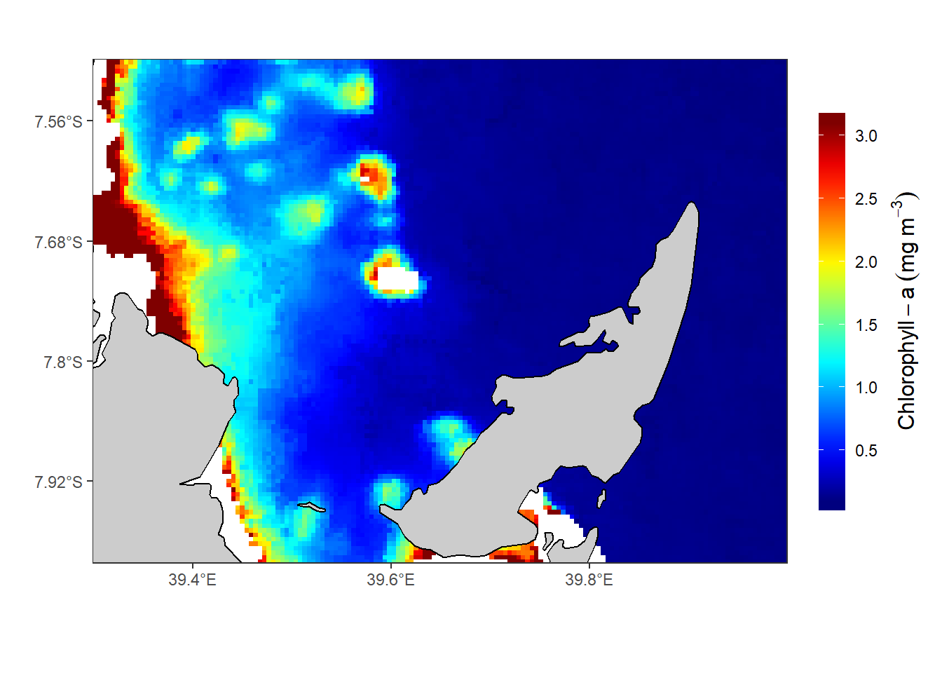

Figure 1: The Spatial distribution of chl-a in the Rufiji-Mafia channel mapped with the ggplot2 package

There are big difference of the chl-values processed with the nc2raster() function from oceanmap package (figure 1) compared to those manipulated with ncdf4 package (figure 2) and raster package (Figure 3). I will explain this differences in the comming posts

ncdf4

## read and open the nc file
chl = ncdf4::nc_open("e:/GIS/Joeline satellite data/Chl-a/M2012092-2012121.vw.all_products.MYO.median.01apr12-30apr12.1368530290.data.nc")

## extract variables
chl.a = ncdf4::ncvar_get(nc = chl, varid = "chl_oc3")
lon = ncdf4::ncvar_get(nc = chl, varid = "longitude")
lat = ncdf4::ncvar_get(nc = chl, varid = "latitude")

## convert the matrix and vector to data frame with expand grid
chl.a.tb = expand.grid(lon,lat) %>% 
  bind_cols(chl.a %>% expand.grid()) %>% 
  as_tibble() %>%
  rename(lon = 1, lat = 2, chl = 3) %>%
  filter(lon >= 39.0 & lon <= 40.0 & lat >= -8.0 & lat <= -7.5 & chl < 4.1)

## map the distribution
ggplot() + 
  geom_raster(data = chl.a.tb, aes(x = lon,  y = lat, fill = chl))+
  geom_sf(data = bongo, fill = "grey80", col = "black")+
  coord_sf(xlim = c(39.29841, 39.99928), c(-8.001797, -7.498381))+
  scale_fill_gradientn(colours = oce::oce.colorsJet(120), na.value = "white", breaks = seq(0,4.2,0.5))+
  metR::scale_x_longitude(ticks = .2) + 
  metR::scale_y_latitude(breaks = c(-7.92, -7.80, -7.68, -7.56))+
  guides(fill = guide_colorbar(title = expression(Chlorophyll-a~(mg~m^{-3})),
                               title.position = "right",
                               title.theme = element_text(angle = 90), 
                               barwidth = unit(.5, "cm"),barheight = unit(7.5, "cm"),title.hjust = .5))+
  theme_bw()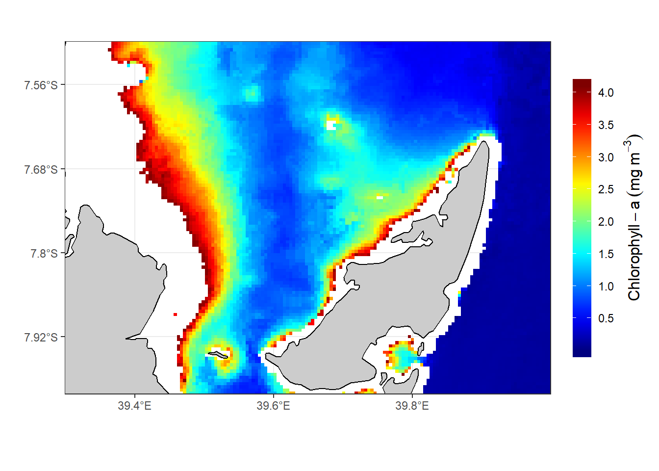

Figure 2: The Spatial distribution of chl-a in the Rufiji-Mafia channel. The chl-a value were procesed using algorithm in ncdf4 package

raster package

## read as raster object
chl.a = raster::raster("e:/GIS/Joeline satellite data/Chl-a/M2012092-2012121.vw.all_products.MYO.median.01apr12-30apr12.1368530290.data.nc", 
                       varname = "chl_oc3")

## create chopping object
rufiji.extent = raster::extent(39.0, 40.0, -8.0,-7.5)
## chop the raster object
chl.a = raster::crop(x = chl.a, y = rufiji.extent) 


#assign all cells with values greater than 4.1 to NA
chl.a = chl.a %>% 
  raster::clamp(upper = 4.1, # lower clamp value
                lower = 0.1,  # upper clamp value
                usevalues = FALSE # force value to NA
                )

## convert from raster object to data frame and then tibble
chl.a.tb = chl.a %>% 
  raster::as.data.frame(xy = TRUE) %>% 
  as_tibble() %>%
  rename(lon = 1, lat = 2, chl = 3) 

## map the distribution of chl
ggplot() + 
  geom_raster(data = chl.a.tb, aes(x = lon,  y = lat, fill = chl))+
  geom_sf(data = bongo, fill = "grey80", col = "black")+
  coord_sf(xlim = c(39.29841, 39.99928), c(-8.001797, -7.498381))+
  scale_fill_gradientn(colours = oce::oce.colorsJet(120), na.value = "white", breaks = seq(0,4.2,0.5))+
  metR::scale_x_longitude(ticks = .2) + 
  metR::scale_y_latitude(breaks = c(-7.92, -7.80, -7.68, -7.56))+
  guides(fill = guide_colorbar(title = expression(Chlorophyll-a~(mg~m^{-3})),
                               title.position = "right",
                               title.theme = element_text(angle = 90), 
                               barwidth = unit(.5, "cm"),barheight = unit(7.5, "cm"),title.hjust = .5))+
  theme_bw()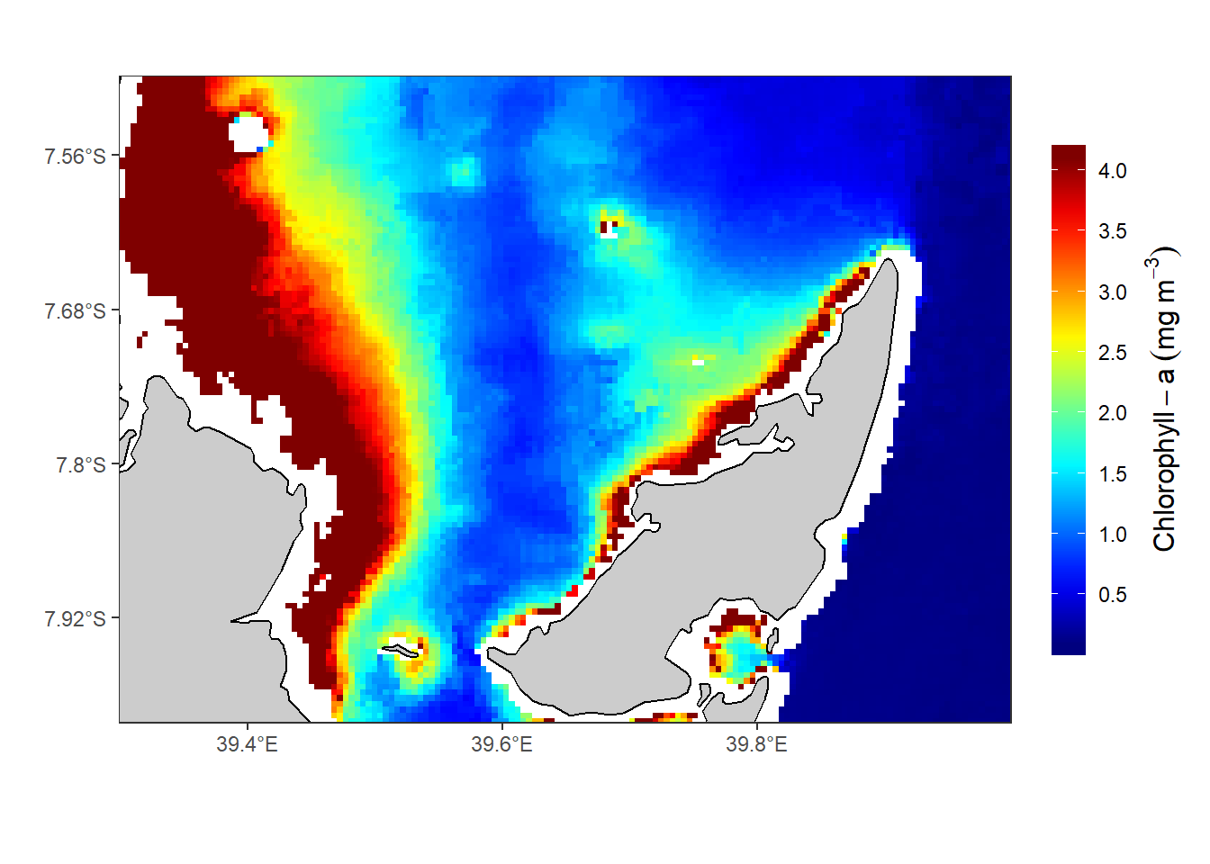

Figure 3: The Spatial distribution of chl-a in the Rufiji-Mafia channel. The chl-a value were procesed using algorithm in raster package