In the previous post, we saw how to make wordcloud graphic using the wordcloud package. In this post we extend the ability of R to make wordcloud graphic, but rather than using the base R function for plotting,I will show how to use ggplot2 framework.
Le Pennec and Slowikowski (2019) developed a gwordcloud package, which extend the capability of ggplot2 package (Wickham 2016) of making cloud text. With the geom_text_wordcloud() function, gwordcloud made making wordcloud plot easy with ggplot2 package. The geom_text_wordcloud() function allows to grow the cloud according to a shape and stay within a mask. The size aesthetic is used either to control the font size or the printed area of the words. ggwordcloud also supports arbitrary text rotation. The faceting scheme of ggplot2 can also be used.
packages
You need functions from various package. You must have these package installed in your machine. To install these package you use the install.packages() function as illustrated in the chunk below;
install.packages("tm")  # for text mining
install.packages("SnowballC") # for text stemming
install.packages("wordcloud") # word-cloud generator
install.packages("RColorBrewer") # color palettes
install.packages("ggwordcloud")
once you have installed these package, you can now load them to make the functions accessible for the task
require("tm")
require("SnowballC")
require("wordcloud")
require("RColorBrewer")
require(tidyverse)
require(magrittr)
require(ggwordcloud)
Data
You need a text file that store the word you need for visualization. For this post I’m going to process the “I have a dream speech” from “Martin Luther King” but you can use any text you want. Since the document is online, I used the read_table() function from readr package.
dream = read_table(file = "http://www.sthda.com/sthda/RDoc/example-files/martin-luther-king-i-have-a-dream-speech.txt",
                   skip_empty_rows = TRUE,
                   progress = TRUE,
                   comment = "" )
Then create a vector source of the text document we downloaded from the internet and transform it to a structure called corpus using vectorSource() and Corpus() function from the tm package (Feinerer, Hornik, and Meyer 2008).
# Load the data as a corpus
# docs = Corpus(VectorSource(dream))

dream.corpus = dream  %>%
  tm::VectorSource()%>%
  tm::Corpus()
Once the corpus file is create, the inspect() function from tm package is used to show detailed information on a corpus document.
dream.corpus %>% inspect()after converting to corpus dataset, we notice that some data cleaning is required. It appears from the earlier data inspection that there are many English words that we need to trim them off and retain only meaningful words. Remove words that include;
- Numerical digits (0–9)
- Stop words, which are common English words like a and the. If you do not remove from the dataset, they dominate the word cloud over the meaningful words
- remove punctuation and extra white space
The whole process is chained using the %>% operator from magritr package
dream.corpus.clean =  dream.corpus %>%
  tm_map(FUN = content_transformer(tolower)) %>% # Convert the text to lower case
  tm_map(FUN = removeNumbers) %>% # Remove numbers
  tm_map(removeWords, stopwords("english")) %>% # Remove english common stopwords
  tm_map(removeWords, c("will", "let", "ring")) %>%   # Remove words
  tm_map(removePunctuation) %>%   # Remove punctuations
  tm_map(stripWhitespace)   # Eliminate extra white spaces
dream.corpus.clean %>% tm::inspect()Build a word frequency table
Once we have a clean, the function TermDocumentMatrix() from tm package (Feinerer, Hornik, and Meyer 2008) was used to make a matrix. Once the matrix is created is converted to data frame with as.data.frame() and pull the rownames into a data frame with the rownames_to column() function from tibble package (Müller and Wickham 2018). And finalize the wrangling with the rename() and arrange() function from dplyr package (Wickham et al. 2018).
dream.corpus.clean.tb=  dream.corpus.clean %>%
  tm::TermDocumentMatrix() %>%
  as.matrix() %>% as.data.frame() %>%
  tibble::rownames_to_column() %>%
  dplyr::rename(word = 1, freq = 2) %>%
  dplyr::arrange(desc(freq))
ggplot(data = dream.corpus.clean.tb,
aes(label = word, size = freq, col = as.character(freq))) +
geom_text_wordcloud(rm_outside = TRUE, max_steps = 1,
grid_size = 1, eccentricity = .9)+
scale_size_area(max_size = 14)+
scale_color_brewer(palette = "Paired", direction = -1)+
theme_void()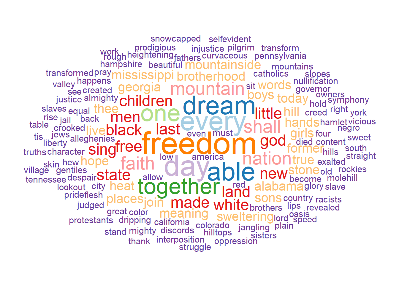
The words can be rotated by setting the angle aesthetic. For instance, one can use a rotation of 90 degrees for a random subset of 40 % of the words:
 dream.corpus.clean.tb = dream.corpus.clean.tb %>%
   mutate(angle = 90 * sample(c(0, 1), n(), replace = TRUE, prob = c(60, 40)))

ggplot(data = dream.corpus.clean.tb,
       aes(label = word, size = freq, angle = angle, col = as.character(freq))) +
  geom_text_wordcloud(rm_outside = TRUE, max_steps = 1,
                      grid_size = 1, eccentricity = .9)+
  scale_size_area(max_size = 14)+
  scale_color_brewer(palette = "Paired", direction = -1)+
  theme_void()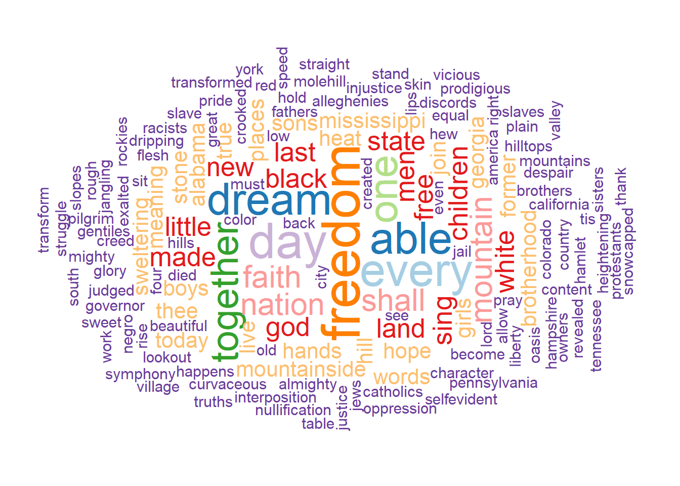
References
Feinerer, Ingo, Kurt Hornik, and David Meyer. 2008. “Text Mining Infrastructure in R.” Journal of Statistical Software 25 (5): 1–54. http://www.jstatsoft.org/v25/i05/.
Le Pennec, Erwan, and Kamil Slowikowski. 2019. Ggwordcloud: A Word Cloud Geom for ’Ggplot2’. https://CRAN.R-project.org/package=ggwordcloud.
Müller, Kirill, and Hadley Wickham. 2018. Tibble: Simple Data Frames. https://CRAN.R-project.org/package=tibble.
Wickham, Hadley. 2016. Ggplot2: Elegant Graphics for Data Analysis. Springer-Verlag New York. http://ggplot2.org.
Wickham, Hadley, Romain François, Lionel Henry, and Kirill Müller. 2018. Dplyr: A Grammar of Data Manipulation. https://CRAN.R-project.org/package=dplyr.