Scientist often store most of oceanographic and environmental variables from satellite sensors in netCDF format. The netCDF data file format contain one or more variables, which are usually structured as regular arrays and metadata describing the contents and format of the data. For example, you might have a variable named “Temperature” that is a function of longitude, latitude, and depth. NetCDF files also contain dimensions, which describe the extent of the variables’ arrays. In our Temperature example, the dimensions are longitude, latitude, and depth. R has a ncdf4 package that allows to read and write netCDF files and its outputs are either array or matrix for the data and atomic vector for other variables like the longitude, latitude, time and depth (Pierce, 2017).
Unfortunately, neither array nor matrix are the fundamental data storage in R. Instead data table is the primary data storage and its this structure that R like to wrange data— manipulation, transformation, analysis. Similarly, most plotting package use data frame for drawing plots pretty easy. In this post, I will ride you through the routine of reading netCDF file and convert it to data frame with raster package. We start by loading the packages we need for this task.
require(sf)
require(tidyverse)
require(raster)
1. read the nc file
Apart from creating from scratch raster layer from matrix or image, a raster() function from raster package can also read the netCDF files and create a raster layer. We use the sea level anomaly data downloaded from AVISO.
sla = raster("./Altimetry/msla_h/indian_ocean-twosat-msla-h_010193_311295.nc",
             level = 180,
             varname = "sla")
2. define projection
Because the data is within the world area, we ought to set the projection. Bivand, Pebesma, Gomez-Rubio, & Pebesma (2008) developed sp package that has proj4string() function, which was used to transform the coordinates of the raster layer to the World Geodetic System (“WGS84”).
proj4string(sla)=CRS("+init=EPSG:4326")3. convert to data frame
The last tranformation involves converting raster layer into data frame. The raster layer was transformed into data frame with as.data.frame() function from raster package. The argument xy = TRUE was parsed in the as.data.frame() to ensure that the process returns the longitude and latitude information as well. Table 1 is the random sample of twelve observation of the sea level anomaly of the data frame created
sla.df = raster::as.data.frame(sla, xy = TRUE)

sla.df %>% sample_n(12) %>% kableExtra::kable("html", row.names = FALSE, col.names = c("Longitude", "Latitude", "Sea Level Anomaly"), align = "c", caption = "Random sample of twelve observations showing the sea level anomaly at specific location") %>%
kableExtra::column_spec(column = 1:3, width = "5cm", color = 1)| Longitude | Latitude | Sea Level Anomaly |
|---|---|---|
| 47.875 | -28.375 | 0.1161 |
| 49.375 | 26.875 | NA |
| 88.875 | -20.375 | -0.0055 |
| 67.125 | -71.125 | NA |
| 87.125 | -61.625 | 0.0271 |
| 21.625 | -3.875 | NA |
| 56.625 | -71.125 | NA |
| 102.125 | -16.875 | -0.1538 |
| 99.875 | -35.875 | -0.0123 |
| 92.875 | 14.375 | 0.0905 |
| 42.375 | -2.375 | -0.0317 |
| 52.125 | -44.375 | -0.1258 |
4. Visualize
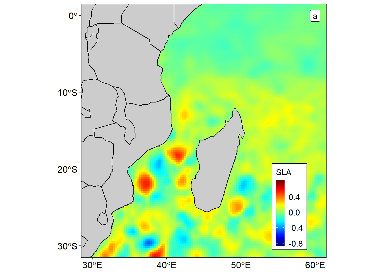
As the data frame is the primary data structure in R (R Core Team, 2018), famous package like tidyverse also depend on tibble—new format of data frame for manipulation and plotting (Wickham, 2017). One of the package of tidyverse is the ggplot2 (Wickham, 2016) that support simple features (E. Pebesma, 2018) for mapping. The sf and *ggplot2** package were used to plot the map of sea level anomaly in figure 1 using data from data frame showin (table 1).
# 4. plot with ggplot using geom_raster function

ggplot()+
  geom_raster(data = sla.df,  aes(x = x, y = y, fill = Sea.Level.Anomalies), interpolate = FALSE)+
  geom_sf(data = spData::world, fill = "grey80", col = "black")+
  # geom_path(data = data, aes(x = lon, y = lat, col = id), size = .75)+
  coord_sf(xlim = c(30, 60), ylim = c(-30, 0))+
  # scale_color_jco(name = "Argo float")+
  theme_bw()+
  theme(legend.position = c(.85,.2),
        legend.background = element_rect(colour = 1),
        legend.key.width = unit(.75, "lines"),
        legend.text = element_text(size = 11, colour = 1),
        axis.text = element_text(colour = 1, size = 12))+
  geom_label(aes(x = 60, y = 0, label = "a"))+
  labs(x = NULL, y = NULL)+
  scale_fill_gradientn(name = "SLA", colours = oce::oceColors9A(120))+
  scale_x_continuous(breaks = seq(30, 60,10))+
  scale_y_continuous(breaks = seq(-30, 5, 10))
Figure 1: Spatial variation of sea level anomalies in the Indian Ocean
Literature
Bivand, R. S., Pebesma, E. J., Gomez-Rubio, V., & Pebesma, E. J. (2008). Applied spatial data analysis with r (Vol. 747248717). Springer.
Pebesma, E. (2018). Sf: Simple features for r. Retrieved from https://CRAN.R-project.org/package=sf
Pierce, D. (2017). Ncdf4: Interface to unidata netCDF (version 4 or earlier) format data files. Retrieved from https://CRAN.R-project.org/package=ncdf4
R Core Team. (2018). R: A language and environment for statistical computing. Vienna, Austria: R Foundation for Statistical Computing. Retrieved from https://www.R-project.org/
Wickham, H. (2016). Ggplot2: Elegant graphics for data analysis. Springer-Verlag New York. Retrieved from http://ggplot2.org
Wickham, H. (2017). Tidyverse: Easily install and load the ’tidyverse’. Retrieved from https://CRAN.R-project.org/package=tidyverse