Creating wordcloud with wordcloud package in R

Why You Would Use word clouds ?

Wordcloud is used in various field including;

• Researchers : for reporting qualitative data
• Marketers : for highlighting the needs and pain points of customers
• Educators : to support essential issues
• Politicians and journalists
• social media sites : to collect, analyze and share user sentiments

packages

You need functions from various package. You must have these package installed in your machine. To install these package you use the install.packages() function as illustrated in the chunk below;

install.packages("tm")  # for text mining
install.packages("SnowballC") # for text stemming
install.packages("wordcloud") # word-cloud generator 
install.packages("RColorBrewer") # color palettes

once you have installed these package, you can now load them to make the functions accessible for the task

require("tm")
require("SnowballC")
require("wordcloud")
require("RColorBrewer")
require(tidyverse)
require(magrittr)

Data

You need a text file with word that you need to make plot. For this post I process the “I have a dream speech” from “Martin Luther King” but you can use any text you want. Since the document is online, I used the read_table() function from readr package.

dream = read_table(file = "http://www.sthda.com/sthda/RDoc/example-files/martin-luther-king-i-have-a-dream-speech.txt", 
                   skip_empty_rows = TRUE,
                   progress = TRUE, 
                   comment = "" )

Then create a vector source of the text document we downloaded from the internet and transform it to corpus using vectorSource() and Corpus() function from the tm package (Feinerer, Hornik, and Meyer 2008).

# Load the data as a corpus
# docs = Corpus(VectorSource(dream))

dream.corpus = dream  %>% 
  tm::VectorSource()%>% 
  tm::Corpus()

Once the corpus file is create, the inspect() function from tm package is used to show detailed information on a corpus document.

dream.corpus %>% inspect()

after converting to corpus dataset, we notice that some data cleaning is required. It appears from the earlier data inspection that there are many English words that we need to trim them off and retain only meaningful words. Remove words that include;

• Numerical digits (0–9)
• Stop words, which are common English words like a and the. If you do not remove from the dataset, they will dominate the word cloud over the meaningful words
• remove punctuation and extra white space

The whole process is chained using the %>% operator from magritr package (Bache and Wickham 2014)

dream.corpus.clean =  dream.corpus %>% 
  tm_map(FUN = content_transformer(tolower)) %>% # Convert the text to lower case
  tm_map(FUN = removeNumbers) %>% # Remove numbers
  tm_map(removeWords, stopwords("english")) %>% # Remove english common stopwords
  tm_map(removeWords, c("will", "let", "ring")) %>%   # Remove words 
  tm_map(removePunctuation) %>%   # Remove punctuations
  tm_map(stripWhitespace)   # Eliminate extra white spaces

dream.corpus.clean %>% tm::inspect()

Build a word frequency table

Once we have a clean, the function TermDocumentMatrix() from tm package (Feinerer, Hornik, and Meyer 2008) was used to make a matrix. Once the matrix is created is converted to data frame with as.data.frame() and pull the rownames into a data frame with the rownames_to column() function from tibble package (Müller and Wickham 2018). And finalize the wrangling with the rename() and arrange() function from dplyr package (Wickham et al. 2018).

dream.corpus.clean.tb=  dream.corpus.clean %>% 
  tm::TermDocumentMatrix() %>% 
  as.matrix() %>% as.data.frame() %>% 
  tibble::rownames_to_column() %>%
  dplyr::rename(word = 1, freq = 2) %>%
  dplyr::arrange(desc(freq))

Once the data is the right format, We plot the wordcloud with the wordcloud() function from wordcloud package (Fellows 2018).

dream.corpus.clean.tb %$% 
  wordcloud::wordcloud(words = word, freq = freq,min.freq = 1, max.words = 200,
                       random.order = FALSE, rot.per = 0.35, colors = brewer.pal(8, "Dark2"))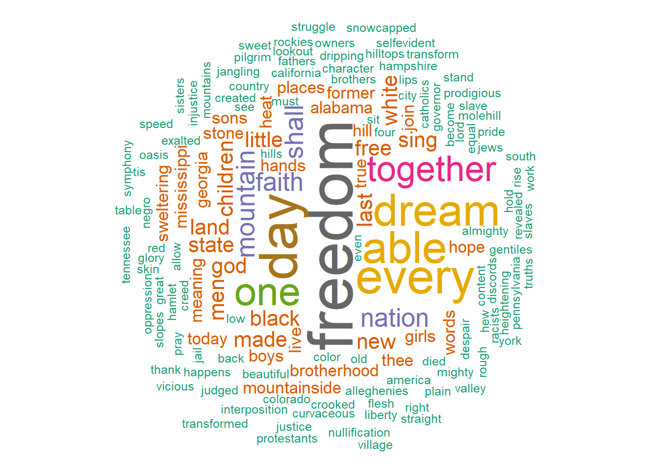

Visualize the wordcloud graphic we get some key insights—The word freedom stands out compare to other words in the speech of Martin Luther King Junior on his speach of I have a dream

References

Bache, Stefan Milton, and Hadley Wickham. 2014. Magrittr: A Forward-Pipe Operator for R. https://CRAN.R-project.org/package=magrittr.
Feinerer, Ingo, Kurt Hornik, and David Meyer. 2008. “Text Mining Infrastructure in R.” Journal of Statistical Software 25 (5): 1–54. http://www.jstatsoft.org/v25/i05/.
Fellows, Ian. 2018. Wordcloud: Word Clouds. https://CRAN.R-project.org/package=wordcloud.
Müller, Kirill, and Hadley Wickham. 2018. Tibble: Simple Data Frames. https://CRAN.R-project.org/package=tibble.
Wickham, Hadley, Romain François, Lionel Henry, and Kirill Müller. 2018. Dplyr: A Grammar of Data Manipulation. https://CRAN.R-project.org/package=dplyr.