quikscat
In his An Introduction to the Near–Real–Time QuikSCAT Data, Hoffman (2005) described the primary mission of the SeaWinds instrument on the National Aeronautics and Space Administration (NASA) Quick Scatterometer (QuikSCAT ) satellite was to retrieve the surface vector wind over the global ocean (Lungu 2001).
QuikSCAT has provided an extremely accurate and extraordinarily comprehensive view of the surface wind over the global ocean since July 1999 (Chelton et al. 2004). With an 1800-km-wide swath, QuikSCAT observations cover 90% of the earth every 24 h.
QuikSCAT data depict the ocean surface wind field, and to provide some insight into the data errors. However, the optimal use of QuikSCAT winds requires proper processing of the data. his
The prime goal of this post is to illustrate how to fetch quikscat wind data with xtractomatic package in R (R Core Team, 2018). Then we will look tools that help us to manipulate, transform and visualize wind data both as smooth raster and arrow vector—direction and speed. We need to load some packages we will use for this analytical procedure..
require(xtractomatic)
require(tidyverse)
require(oce)
require(lubridate)
require(gganimate)
require(sf)
The SeaWinds on QuikSCAT Level 3 data set consists of gridded values of scalar wind speed, meridional and zonal components of wind velocity, wind speed squared and time given in fraction of a day. The SeaWinds on QuikSCAT Level 3 Daily, Gridded Ocean Wind Vectors data set is available at ERDDAP servers. the dataset ids for zonal is qsux101day and meridional is qsux101day. we can check the metadata information for these datasets with getinfo() function from xtractomatic package
getInfo("qsux101day")
getInfo("qsuy101day")
We define the tropical Indian Ocean region as geographical boundary and the year 2006 as the time bound
# set spatial extent
lon = c(25,65)
lat =  c(-35,10)
## set temporal extent
time = c("2006-01-01", "2006-12-31")
The the dataset id, spatial and time bounds were passed in the extracto_3D() function as argument to extract and download quikscat data based. Because we want the vector wind fields, the zonal and meridional data were download separately.
wind_x = xtracto_3D(dtype = "qsux101day",
                    xpos = lon,
                    ypos = lat,
                    tpos = time)

wind_y = xtracto_3D(dtype = "qsuy101day",
                    xpos = lon,
                    ypos = lat,
                    tpos = time)
The downloaded dataset contain vecotr array of zonal and meridional wind speed velocity along with longitudes, latitudes and times. To obtain these information we first extract location and time bounds as vector
## extract location and time bounds as vector
longitude = wind_x$longitude
latitude = wind_x$latitude
time = wind_x$time%>%as.Date()
The wind field for eastward velocity (U) and northward velocity (V) were exracted as array and compute the velocity of wind speed from these arrays. Each array contain a list of 365 matrices—each matrix contain wind field of a single day.
## extract u and v as array
# eastward velocity (zonal)
u = wind_x$data
# northward velocity (meridional)
v = wind_y$data

# calculate wind velocity
velocity = sqrt(u^2 + v^2)
Converting array to data frame.
Most data analyis in R works with data frame (R Core Team, 2018) that are tidy—organize the data that each variable is a column and each observation is a row. Its the tidy data that provide easy data cleaning, modeling and visualization. The tidyr package by Hadley Wickham is designed to help tidy the data (Wickham & Henry, 2018). It contains four functions that alter the layout of tabular data sets, while preserving the values and relationships contained in the data sets. The two most important functions in tidyr are gather() and spread(). Therefore, the arrays were transformed and tidy to data frame. Because there are 365 matrix for each array, it is tidious to tranform them to data frame manually. I used the for() loop function to iterate the process.
n.lon = length(longitude)
n.lat = length(latitude)+1

u.all = NULL

for (i in 1:length(time)){
      u.df = data.frame(longitude, u[,,i] %>% as.data.frame()) %>%
        gather(key = "key" , value = "u", 2:n.lat) %>%
        mutate(latitude = rep(latitude, each = n.lon), date = time[i]) %>%
        select(date,longitude, latitude, u)%>%
        as.tibble()

    u.all = u.all %>% bind_rows(u.df)
}
v.all = NULL
for (i in 1:length(time)){
v.df = data.frame(longitude, v[,,i] %>% as.data.frame()) %>%
gather(key = "key" , value = "v", 2:n.lat) %>%
mutate(latitude = rep(latitude, each = n.lon), date = time[i]) %>%
select(date,longitude, latitude, v)%>%
as.tibble()
v.all = v.all %>% bind_rows(v.df)
}velocity.all = NULL
for (i in 1:length(time)){
velocity.df = data.frame(longitude, velocity[,,i] %>% as.data.frame()) %>%
gather(key = "key" , value = "velocity", 2:n.lat) %>%
mutate(latitude = rep(latitude, each = n.lon), date = time[i]) %>%
select(date,longitude, latitude, velocity)%>%
as.tibble()
velocity.all = velocity.all %>% bind_rows(velocity.df)
}Wind Fields Manipulation
After converting the array into data frame, we can manipulate the data based on daily, weekly and monthly. Here we compute the monthly zonal, meridional and velocity wind observations into main steps. First, because we do not deal with the entire region, we selected data for the area of interest by define the geographical bounds with filter() function. Second, the date variable was decomposed into day, week and month variables. Third, latitude, longitude was aggregated by month and computed the monthly mean of zonal meridional and velocity with summarise() function.
velocity.month = velocity.all %>%
  filter(between(longitude,38,55)) %>%
  filter(between(latitude,-15,-7)) %>%
  mutate(day = yday(date) %>% as.integer(), week = week(date)%>% as.integer(),
         month = month(date)%>% as.integer())%>%
  group_by(longitude, latitude, month) %>%
  summarise(velocity = mean(velocity, na.rm = TRUE))

u.month = u.all %>%
  filter(between(longitude,38,55)) %>%
  filter(between(latitude,-15,-7)) %>%
  mutate(day = yday(date) %>% as.integer(), week = week(date)%>% as.integer(),
         month = month(date)%>% as.integer()) %>%
  group_by(longitude, latitude, month) %>%
  summarise(u = mean(u, na.rm = TRUE))

v.month = v.all %>%
  filter(between(longitude,38,55)) %>%
  filter(between(latitude,-15,-7)) %>%
  mutate(day = yday(date) %>% as.integer(), week = week(date)%>% as.integer(),
         month = month(date)%>% as.integer()) %>%
  group_by(longitude, latitude, month) %>%
  summarise(v = mean(v, na.rm = TRUE))
Once the monthly winded fields were computed, its time to tidy them into a single data frame. The files—u.month, v.month and velocity.month were binded by column with a bind_cols() function and select variable of interest and ungrouped the data frame.
month.wind.vector = velocity.month %>%
  bind_cols(u.month, v.month) %>%
  select(longitude, latitude, month, u,v,velocity) %>%
  ungroup()
Monsoon winds influence the region and this is clearly in figure (fig:fig1). The northeast expreience week wind (Figure (fig:fig1)a of February 2006 compared to a strong wind during the southeast monsoon winds (Figure (fig:fig1)b) of August 2006.
feb = ggplot(data = month.wind.vector %>% filter(month == 2)) +
  geom_raster(aes(x = longitude, y = latitude, fill = velocity))+
  scale_fill_gradientn(limits = c(0,15),colours = oceColorsPalette(120),
                       na.value = "white", name = "Speed\n(m/s)")+
  geom_sf(data = spData::world, fill = "grey85", col = "black")+
  coord_sf(xlim = c(39,54), ylim = c(-14.5,-7.5))+
  theme_bw()+
  theme(axis.text = element_text(size = 11, colour = "black"))+
  labs(x = NULL, y = NULL)

aug = ggplot(data = month.wind.vector %>% filter(month == 8)) +
  geom_raster(aes(x = longitude, y = latitude, fill = velocity))+
  scale_fill_gradientn(limits = c(0,15),colours = oceColorsPalette(120),
                       na.value = "white", name = "Speed\n(m/s)")+
  geom_sf(data = spData::world, fill = "grey85", col = "black")+
  coord_sf(xlim = c(39,54), ylim = c(-14.5,-7.5))+
  theme_bw()+
  theme(axis.text = element_text(size = 11, colour = "black"))+
  labs(x = NULL, y = NULL)

cowplot::plot_grid(feb,aug, nrow = 2, labels = c("a)", "b)"), label_x = .7, label_y = .94, label_size = 12)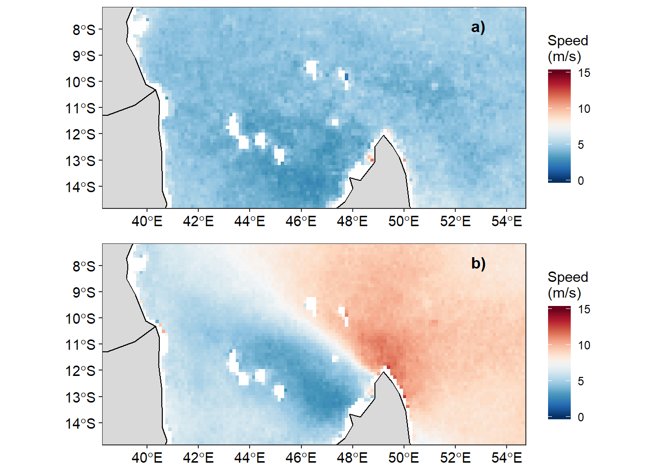
Figure 1: Wind speed a) February 2006 and b) August 2006
The development of the wind is much clear when the twelve month are drawn in sequantial order (figure 2)
ggplot(data = month.wind.vector) +
  geom_raster(aes(x = longitude, y = latitude, fill = velocity))+
  scale_fill_gradientn(limits = c(0,15),colours = oceColorsPalette(120),
                       na.value = "white", name = "Speed\n(m/s)")+
  geom_sf(data = spData::world, fill = "grey85", col = "black")+
  coord_sf(xlim = c(39,54), ylim = c(-14.5,-7.5))+
  theme_bw()+
  theme(axis.text = element_text(size = 11, colour = "black"))+
  scale_x_continuous(breaks = c(42,52))+
  scale_y_continuous(breaks = c(-14,-8))+
  labs(x = NULL, y = NULL)+
  facet_wrap(~month, ncol = 3)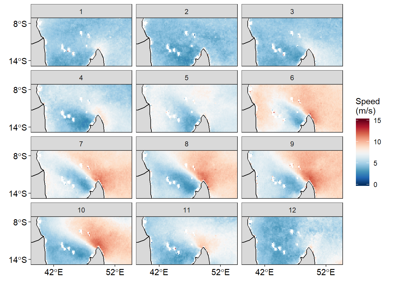
Figure 2: Monthly wind velocity for the year 2006
Figure 3 illustrate the animated monthly wind velocity similar to figure 2.
ggplot(data = month.wind.vector) +
  geom_raster(aes(x = longitude, y = latitude, fill = velocity))+
  scale_fill_gradientn(limits = c(0,15),colours = oceColorsPalette(120),
                       na.value = "white", name = "Speed\n(m/s)")+
  geom_sf(data = spData::world, fill = "grey85", col = "black")+
  coord_sf(xlim = c(39,54), ylim = c(-14.5,-7.5))+
  theme_bw()+
  theme(axis.text = element_text(size = 11, colour = "black"))+
  labs(x = NULL, y = NULL)+
    #animate
  labs(title = 'Month: {frame_time}') +
  transition_time(month) +
  ease_aes('linear')
Figure 3: Animated monthly wind velocity
make grid
Overalying the vector wind speed and direction on the wind velocity make the plot a messy. This is because the vector fields and velocity are high resolution and arrow clutter when plotted (figure 4). This make the plot unpleasant and we need to reduce the number of vector fields.
ggplot(data = month.wind.vector %>% filter(month == 8)) +
  geom_raster(aes(x = longitude, y = latitude, fill = velocity))+
  scale_fill_gradientn(limits = c(0,15),colours = oceColorsPalette(120),
                       na.value = "white", name = "Speed\n(m/s)")+
  geom_segment(aes(x = longitude, xend = longitude+u/10, y = latitude, yend = latitude+v/10),
               arrow = arrow(length = unit(0.2, "cm")))+
  geom_sf(data = spData::world, fill = "grey85", col = "black")+
  coord_sf(xlim = c(39,54), ylim = c(-14.5,-7.5))+
  theme_bw()+
  theme(axis.text = element_text(size = 11, colour = "black"))+
  labs(x = NULL, y = NULL)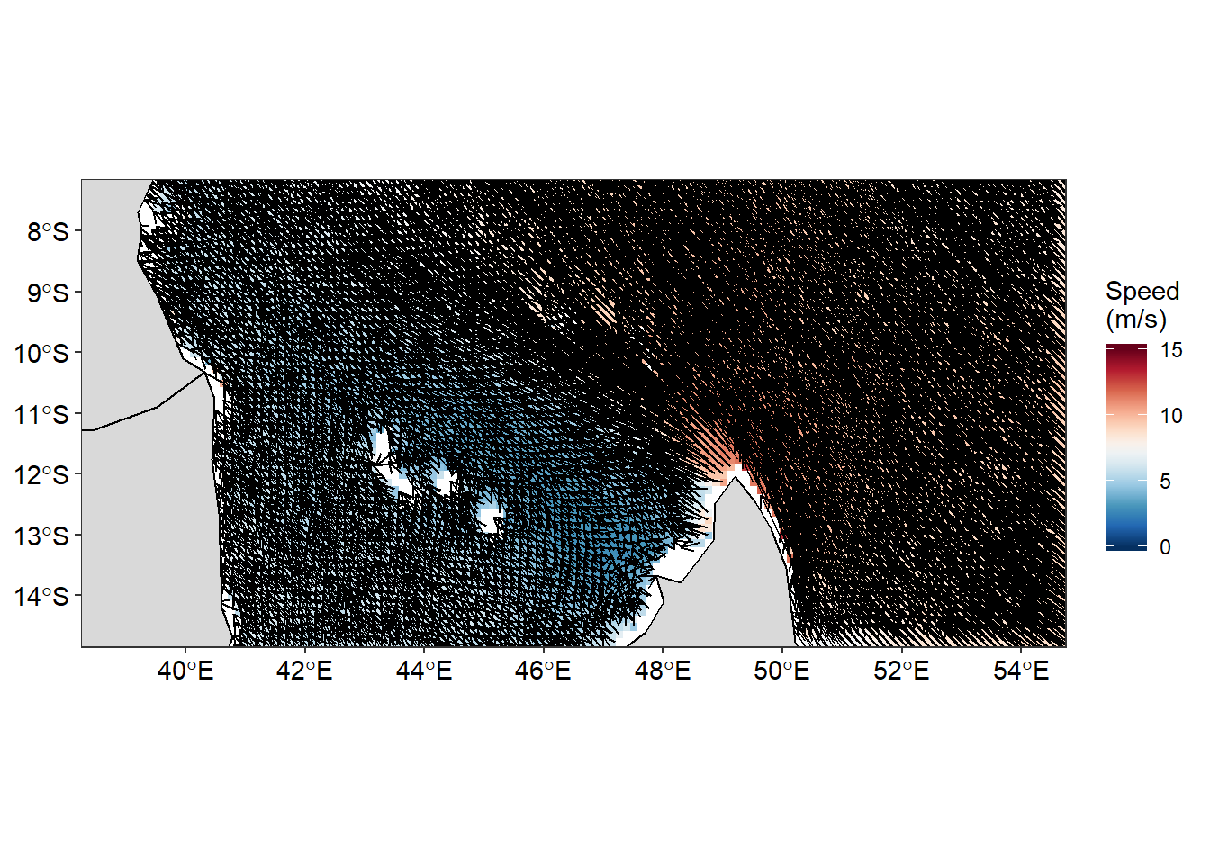
Figure 4: Wind speed and direction overlaid on wind velocity
that good, we need to grid them and then overlay on the velocity map
require(sf)
require(spData)
data("world")

## make an extent polygone by interactive drawing with the mapview and editmap packages
# extent = mapview::mapview(world)%>%mapedit::editMap()
# extent = extent$drawn

#read extent data w
extent = read_sf("E:/Data Manipulation/xtractomatic/extent.shp")

grid = extent %>%
  st_make_grid(n = c(30,20)) %>%
  st_sf()

# mapview::mapview(grid)
Unlike dataframe, where you can stitch by rows a data frame with NULL() Object, binding sf object and NULL() object will fail. Ttherefore, we must create the simple feature for january first outside the loop and then the looping begin from February and stitch february data to january. The subsequent month data will stitch without problem.
## transform monthly month.wind.vector from tabular form to simple feature
month.wind.vector.sf = month.wind.vector %>%
  st_as_sf(coords = c("longitude", "latitude")) %>%
  st_set_crs(4326)

 ## select the simple point for January.
wind.sf = month.wind.vector.sf %>% filter(month == 1)

## grid the observations and calculate the median of u, v, and velocity in each grid
grid.wind.month = grid %>% mutate(id = n(),
                contained = lapply(st_contains(st_sf(geometry),wind.sf), identity),
                obs = sapply(contained, length),
                u = sapply(contained, function(x) {median(wind.sf[x,]$u, na.rm = TRUE)}),
                v = sapply(contained, function(x) {median(wind.sf[x,]$v, na.rm = TRUE)}),
                velocity = sapply(contained, function(x) {median(wind.sf[x,]$velocity, na.rm = TRUE)}))
## select the u , v and velocity variable and add a month column
grid.wind.month = grid.wind.month %>% select(obs, u, v, velocity) %>% mutate(month = 1)

## that is for january, now loop through from February to December, after each loop, the observation are added in the January values in row order
for (i in 2:12){
wind.sf = month.wind.vector.sf %>% filter(month == i)

leo = grid %>% mutate(id = n(),
                contained = lapply(st_contains(st_sf(geometry),wind.sf), identity),
                obs = sapply(contained, length),
                u = sapply(contained, function(x) {median(wind.sf[x,]$u, na.rm = TRUE)}),
                v = sapply(contained, function(x) {median(wind.sf[x,]$v, na.rm = TRUE)}),
                velocity = sapply(contained, function(x) {median(wind.sf[x,]$velocity, na.rm = TRUE)}))

leo = leo %>% select(obs, u, v, velocity) %>% mutate(month = i)

grid.wind.month = grid.wind.month %>% rbind(leo)

}
Transform grid to data frame
As mentioned in previous section, the fundamental of data analysis in R rely on data frame. The grids were transformed into data frame. The process involved obtaining the centorid position of grids with st_centroid() and extract the coordinates of the centroid with st_coordinates(). These coordinates were then converted into data frame. The attributes of the grids were then combined with the coordinates of the grids to make a data frame with geograhical location and wind vector fields - zonal, meridional and velocity (table 1)
## create the centroid coordinates from the grids and rename the coordinates
grid.wind.points = grid.wind.month %>%
  st_centroid() %>%
  st_coordinates() %>%
  as.tibble() %>%
  rename(longitude = X, latitude = Y)

## make  a copy of the grid.wind.month
attributes = grid.wind.month
## remove the geometry and remain with the attributes
st_geometry(attributes) = NULL

## bind grid cooordinates with the attributes information
gridded.wind = grid.wind.points %>% bind_cols(attributes)

gridded.wind %>%
  sample_n(15) %>%
  kableExtra::kable("html", caption = "Wind vector fields", align = "c", digits = 4) %>%
kableExtra::column_spec(column = 1:7, width = "4cm",color = "black")| longitude | latitude | obs | u | v | velocity | month |
|---|---|---|---|---|---|---|
| 40.2283 | -9.3221 | 20 | -4.6500 | 0.7964 | 5.0729 | 10 |
| 56.2317 | -14.4064 | 0 | NA | NA | NA | 6 |
| 52.7527 | -9.8305 | 20 | -5.1807 | 6.6102 | 9.0126 | 6 |
| 50.6653 | -12.8811 | 24 | -3.7530 | 4.4700 | 6.8701 | 5 |
| 51.3611 | -13.8979 | 20 | -4.8380 | 6.7907 | 8.9086 | 6 |
| 38.8367 | -13.3895 | 24 | NA | NA | NA | 3 |
| 43.0115 | -12.8811 | 20 | -2.0750 | 0.2051 | 4.1057 | 11 |
| 56.2317 | -7.2884 | 0 | NA | NA | NA | 5 |
| 52.0569 | -7.7968 | 24 | -4.6448 | 7.2017 | 9.0062 | 6 |
| 40.9241 | -11.8642 | 24 | -1.9765 | 4.1506 | 6.2018 | 4 |
| 52.7527 | -6.2716 | 0 | NA | NA | NA | 7 |
| 53.4485 | -7.7968 | 24 | -3.9798 | 3.7350 | 6.2342 | 5 |
| 42.3157 | -8.8137 | 24 | -3.9338 | 3.3237 | 6.0334 | 4 |
| 39.5325 | -13.8979 | 24 | NA | NA | NA | 7 |
| 41.6199 | -13.3895 | 20 | -2.3658 | 3.8161 | 5.9606 | 8 |
Figure 5 show the wind speed and direction. The influence of monsoon winds is much clear in this area. The northeast expreience week wind (Figure (fig:fig5)a of February 2006 compared to a strong wind during the southeast monsoon winds (Figure (fig:fig5)b) of August 2006.
feb = ggplot(data = month.wind.vector %>% filter(month == 2)) +
  geom_raster(aes(x = longitude, y = latitude, fill = velocity))+
  scale_fill_gradientn(limits = c(0,15),colours = oceColorsPalette(120),
                       na.value = "white", name = "Speed\n(m/s)")+
  geom_segment(data = gridded.wind%>% filter(month == 2),
               aes(x = longitude, xend = longitude+u/10, y = latitude, yend = latitude+v/10),
               arrow = arrow(length = unit(0.2, "cm")))+
  geom_sf(data = spData::world, fill = "grey85", col = "black")+
  coord_sf(xlim = c(39,54), ylim = c(-14.5,-7.5))+
  theme_bw()+
  theme(axis.text = element_text(size = 11, colour = "black"))+
  labs(x = NULL, y = NULL)

aug = ggplot(data = month.wind.vector %>% filter(month == 8)) +
  geom_raster(aes(x = longitude, y = latitude, fill = velocity))+
  scale_fill_gradientn(limits = c(0,15),colours = oceColorsPalette(120),
                       na.value = "white", name = "Speed\n(m/s)")+
  geom_segment(data = gridded.wind%>% filter(month == 8),
               aes(x = longitude, xend = longitude+u/10, y = latitude, yend = latitude+v/10),
               arrow = arrow(length = unit(0.2, "cm")))+
  geom_sf(data = spData::world, fill = "grey85", col = "black")+
  coord_sf(xlim = c(39,54), ylim = c(-14.5,-7.5))+
  theme_bw()+
  theme(axis.text = element_text(size = 11, colour = "black"))+
  labs(x = NULL, y = NULL)

cowplot::plot_grid(feb,aug, nrow = 2, labels = c("a)", "b)"), label_x = .7, label_y = .94, label_size = 12)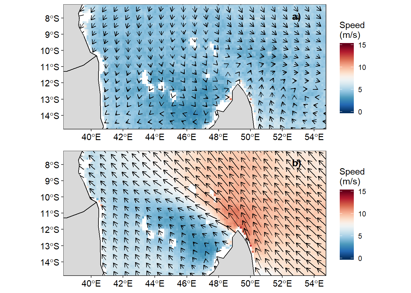
Figure 5: Wind speed and direction overlaid on wind velocity
The animated wind speed and direction of the area is shown in figure 6, which highlight how the wind speed and direction various with months throughtout the year. The animated wind speed and direction shows a much clear picture of the characteristic of winds in this area.
gridded.wind$month = as.integer(gridded.wind$month)

ggplot() +
  geom_raster(data = month.wind.vector, aes(x = longitude, y = latitude, fill = velocity))+
  scale_fill_gradientn(limits = c(0,15),colours = oceColorsPalette(120),
                       na.value = "white", name = "Speed\n(m/s)")+
  geom_segment(data = gridded.wind,
               aes(x = longitude, xend = longitude+u/10, y = latitude, yend = latitude+v/10),
               arrow = arrow(length = unit(0.2, "cm")))+
  geom_sf(data = spData::world, fill = "grey85", col = "black")+
  coord_sf(xlim = c(39,54), ylim = c(-14.5,-7.5))+
  theme_bw()+
  theme(axis.text = element_text(size = 11, colour = "black"))+
  labs(x = NULL, y = NULL)+
    #animate
  labs(title = 'Day: {frame_time}') +
  transition_time(month) +
  ease_aes('linear')
Figure 6: Animate monthly wind speed and direction
bibliography
Hoffman, R. N., & Leidner, S. M. (2005). An introduction to the near–real–time quikscat data. Weather and Forecasting, 20(4), 476–493.
R Core Team. (2018). R: A language and environment for statistical computing. Vienna, Austria: R Foundation for Statistical Computing. Retrieved from https://www.R-project.org/
Wickham, H., & Henry, L. (2018). Tidyr: Easily tidy data with ’spread()’ and ’gather()’ functions. Retrieved from https://CRAN.R-project.org/package=tidyr