The Advanced Scatterometer (ASCAT) winds products are processed by NOAA/NESDIS utilizing measurements from the scatterometer instrument aboard the EUMETSAT Metop satellites. The instrument uses radar to measure backscatter to determine speed and direction of winds over the surface of the oceans. ASCAT observations fields have regular spatial resolutions of 0.25° in longitude and latitude.
The daily wind fields are calculated in near real time with a delay of 48 hours. This first version is considered as data test that will provide useful insight for near real time production of high space and time resolutions at global and regional scales. Daily images are archived for 7 days.
Mendelssohn (2018) developed an xtractomatic package for R that can access ASCAT daily data through The Environmental Research Division’s Data Access Program (ERDDAP).ERDDAP is a simple to use yet powerful web data service developed by Bob Simons (Simons, 2011). The ERDDAP server can also be directly accessed at http://coastwatch.pfeg.noaa.gov/erddap.
The xtractomatic package accesses data that are served through the ERDDAP server at the NOAA/SWFSC Environmental Research Division. This package has ability to subset and extract satellite and other oceanographic related data from a remote server for a moving point in time along a user-supplied set of longitude, latitude and time points; in a 3D bounding box; or within a polygon (through time).
The goal of this post is to illustrate how to fetch satellite wind data collected by ASCAT with xtractomatic package in R (R Core Team, 2018). Then we will look tools that help us to manipulate, transform and visualize wind satellite data. FIrst let us load the packages that holds tools we will use for fetching data manipulate, tranform wind data, and plotting and mapping the results.
require(xtractomatic)
require(tidyverse)
require(oce)
require(lubridate)
require(gganimate)
Ascat
As described in the introduction section, we will use the wind data fo the tropical Indian Ocean area from ASCAT. Because the size of the geographical area and the daily wind data, I will limit the amoung of data to extract to within a period January 01 to October 23, 2018. I will use the xtracto_3D() function to download the wind data. xtracto_3D() extracts wind data within the specified geographical extent. The dataset id for the data are erdQAxwind1day for zonal component and erdQAywind1day for meridional component. You can use the getInfo() function to obtain the metadata of the dataset.
getInfo("erdQAxwind1day")List of 19
$ dtypename : chr "erdQAxwind1day"
$ datasetname : chr "erdQAwind1day"
$ longname : chr "X-Wind, METOP ASCAT, Global, Near Real Time (1 Day Composite) "
$ varname : chr "x_wind"
$ hasAlt : logi TRUE
$ latSouth : logi TRUE
$ lon360 : logi TRUE
$ minLongitude : num 0
$ maxLongitude : num 360
$ longitudeSpacing: num 0.25
$ minLatitude : num -75
$ maxLatitude : num 75
$ latitudeSpacing : num 0.25
$ minAltitude : num 10
$ maxAltitude : num 10
$ minTime : chr "2009-10-03"
$ maxTime : chr "2018-10-23"
$ timeSpacing : num NA
$ infoURL : chr "http://coastwatch.pfeg.noaa.gov/infog/CW_soon_las.html"getInfo("erdQAywind1day")List of 19
$ dtypename : chr "erdQAywind1day"
$ datasetname : chr "erdQAwind1day"
$ longname : chr "Y-Wind, METOP ASCAT, Global, Near Real Time (1 Day Composite) "
$ varname : chr "y_wind"
$ hasAlt : logi TRUE
$ latSouth : logi TRUE
$ lon360 : logi TRUE
$ minLongitude : num 0
$ maxLongitude : num 360
$ longitudeSpacing: num 0.25
$ minLatitude : num -75
$ maxLatitude : num 75
$ latitudeSpacing : num 0.25
$ minAltitude : num 10
$ maxAltitude : num 10
$ minTime : chr "2009-10-03"
$ maxTime : chr "2018-10-23"
$ timeSpacing : num NA
$ infoURL : chr "http://coastwatch.pfeg.noaa.gov/infog/CW_soon_las.html"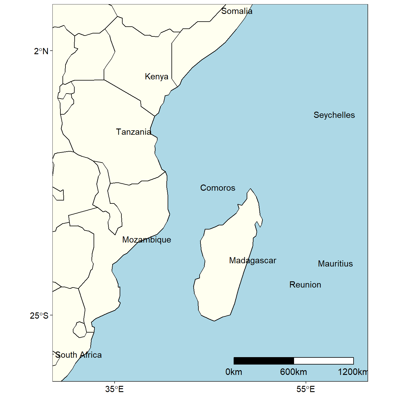
Figure 1: Map of the tropical Western Indian Ocean Region
Using xtracto_3D
First we define the geographical extent and the time limit. Our area of interest is the tropical Indian Ocean region that lies between longitude 25 oE and 65 oE and latitude 35 oS and 10 oN (figure 1). And only interested with the data for 2018, so I set the time limit from January 01, 2018 to the latest data available—October 23, 2018. Be aware R understand YYY-MM-DD time format.
# set spatial extent
lon = c(25,65)
lat =  c(-35,10)
## set temporal extent
time = c("2018-01-01", "2018-10-23")
The extract will contain data at all of the longitudes, latitudes and times in the requested dataset that are within the given bounds.
wind_x = xtracto_3D(dtype = "erdQAxwind1day",
                    xpos = lon,
                    ypos = lat,
                    tpos = time)

wind_y = xtracto_3D(dtype = "erdQAxwind1day",
                    xpos = lon,
                    ypos = lat,
                    tpos = time)
Once the data download has completed, we can check the internal structure of the data with a glimpse() function of dplyr package (Wickham, François, Henry, & Müller, 2018). Glimpsing the file we notice that, apart from the the longitude, latitude and time bounds, there are other information. Thse includes a three-dimension data, variable name and altitude.
glimpse(wind_x)List of 7
$ data : num [1:161, 1:181, 1:296] 17.4 16.6 16.4 15.9 13.9 ...
$ varname : chr "x_wind"
$ datasetname: chr "erdQAwind1day"
$ latitude : num [1:181(1d)] -35 -34.8 -34.5 -34.2 -34 ...
$ longitude : num [1:161(1d)] 25 25.2 25.5 25.8 26 ...
$ time : POSIXlt[1:296], format: "2018-01-01 12:00:00" "2018-01-02 12:00:00" ...
$ altitude : num 10We can extract these variables with $ operator as shown in the chunk below. We obtain the Zonal component and meridional component.
longitude = wind_x$longitude
latitude = wind_x$latitude
time = wind_x$time%>%as.Date()

# eastward velocity (zonal)
u = wind_x$data
# northward velocity (meridional)
v = wind_y$data
Looking the class of the u and v data with class() function, we noticed that they are both array— consisting of a collection of matrix of wind velocity. The eastward velocity (zonal) and northward velocity (v) both have a dimension of 161, 181, 296— of longitude, latitude for 296 days begining from 2018-01-01 to 2018-10-23 . Equation (1) was used to calculate the wind speed from the u and v.
$$ Where \(\phi\) = wind speed; \(u\) = zonal and \(v\) = meridional component of wind
# calculate wind velocity
velocity = sqrt(u^2 + v^2)
Figure 2 show the wind speed within the tropical Indian Ocean on 2018-01-01 There are gaps of missing wind speed values. The plot was generated with imagep() function of oce package (Kelley & Richards, 2018). The nice thing with the imagep() is its ability to plot matrix data.
imagep(longitude,
       latitude,
       velocity[,,1],
       filledContour = TRUE,
       xlab = "Longitude",
       ylab = "Latitude")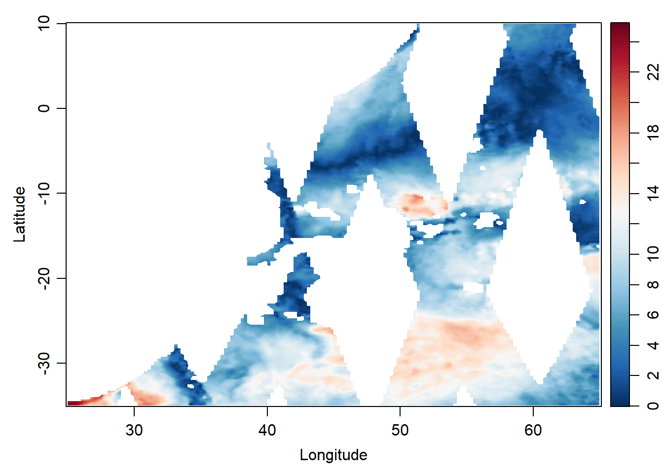
Figure 2: Wind speed of January 1, 2018 in the tropical Indina Ocean
Data frame
Daniel Kelley (???) desribed data frames as a complement to matrices and lists, and they are very important in R. (R Core Team, 2018) states that data frames are fundamental data structure by most of R’s modeling software. Since, data frame is the primary structure for working with data in R, I converted the array into data frame so that I can use the power of tidyverse—a set of packages that provide a useful set of tools for data cleaning and analysis and visualizing (Wickham, 2017).
# convert the first matrix of u component into data frame
u.df = data.frame(longitude, u[,,1] %>% as.data.frame()) %>%
  gather(key = "key" , value = "u", 2:182) %>%
  mutate(latitude = rep(latitude, each = 161), date = time[1]) %>%
  select(date, longitude, latitude, u)%>%
  as.tibble()

# convert the first matrix of v component into data frame
v.df = data.frame(longitude, v[,,1] %>% as.data.frame()) %>%
  gather(key = "key" , value = "v", 2:182) %>%
  mutate(latitude = rep(latitude, each = 161), date = time[1]) %>%
  select(date,longitude, latitude, v)%>%
  as.tibble()

# convert the first matrix of wind speed component into data frame
velocity.df = data.frame(longitude, velocity[,,1] %>% as.data.frame()) %>%
  gather(key = "key" , value = "velocity", 2:182) %>%
  mutate(latitude = rep(latitude, each = 161), date = time[1]) %>%
  select(date,longitude, latitude, velocity)%>%
  as.tibble()
Figure 3 is similar to figure 2 the only difference is the tools used. While Figure 2 was drawn with imagep() of oce package, figure 3 was plotted with ggplot2—a package of tidyverse.
ggplot() +
  geom_raster(data = velocity.df %>% na.omit(),
              aes(x = longitude, y = latitude, fill = velocity), interpolate = FALSE)+
  geom_sf(data = spData::world, col = "black", fill = "ivory")+
  coord_sf(xlim = c(30,65), ylim =  c(-30,5))+
  scale_fill_gradientn(limits = c(0,25), name = "Wind\nSpeed\n(m/s)",
                       colours = oceColorsPalette(120))+
  theme_bw()+
  theme(panel.background = element_rect(fill = "white"),
        axis.text = element_text(size = 11, colour = 1),
        panel.grid = element_line(colour = NA),
        legend.position = c(.1,.25),
        legend.background = element_rect(colour = NA, fill = "ivory"))+
  scale_x_continuous(breaks = c(35,55))+
  scale_y_continuous(breaks = c(-25, 2)) +
  ggsn::scalebar(location = "bottomright", x.min = 35, x.max = 58,
                 y.min = -30, y.max = 5, dist = 600, dd2km = TRUE,
                 model = "WGS84", st.dist = 0.02, st.size = 4)+
  labs(x = NULL, y = NULL)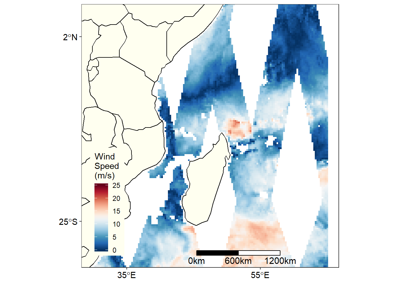
Figure 3: Map showing Wind speed of January 1, 2018 in the tropical Indina Ocean
Loops
The data frame we created above is for single data, however, our dataset has 296 matrix that we need to convert to data frame. To overcome this challenge we loop the process. R has several styles of looping structures that provide for repeated calculation. The chunk below contain the steps for looping the matrix, convert them to data frame etc
velocity.all = NULL

for (i in 1:length(time)){
      velocity.df = data.frame(longitude, velocity[,,i] %>% as.data.frame()) %>%
        gather(key = "key" , value = "velocity", 2:182) %>%
        mutate(latitude = rep(latitude, each = 161), date = time[i]) %>%
        select(date,longitude, latitude, velocity)%>%
        as.tibble()

    velocity.all = velocity.all %>% bind_rows(velocity.df)
}
ncol(velocity.all)
[1] 4The data frame contains 8625736 observations and 4 variables. I used the lubridate package to extract date components from the date variable. These components include the Julian day, the week in a year and month of each observation (Table 1)
velocity.all = velocity.all %>%
  mutate(jd = yday(date), week = week(date), month = month(date)) %>%
  select(date, jd, week, month, longitude, latitude, velocity)

velocity.all%>%
  na.omit()%>%
  sample_n(15) %>%
  kableExtra::kable("html", caption = "Wind speed information in the tropical Indian Ocean",
                  align = "c", digits = 2) %>%
kableExtra::column_spec(column = 1:7, width = "3cm", color = 1)| date | jd | week | month | longitude | latitude | velocity |
|---|---|---|---|---|---|---|
| 2018-08-31 | 243 | 35 | 8 | 39.50 | -25.50 | 10.88 |
| 2018-09-30 | 273 | 39 | 9 | 49.00 | -27.00 | 4.45 |
| 2018-07-08 | 189 | 27 | 7 | 54.50 | -16.50 | 10.99 |
| 2018-02-16 | 47 | 7 | 2 | 56.75 | -28.00 | 7.45 |
| 2018-09-03 | 246 | 36 | 9 | 50.00 | 3.00 | 3.11 |
| 2018-05-11 | 131 | 19 | 5 | 50.50 | -16.50 | 6.04 |
| 2018-01-09 | 9 | 2 | 1 | 59.50 | -21.75 | 7.59 |
| 2018-09-23 | 266 | 38 | 9 | 41.00 | -7.50 | 7.92 |
| 2018-06-29 | 180 | 26 | 6 | 58.25 | -4.25 | 5.85 |
| 2018-07-02 | 183 | 27 | 7 | 62.25 | -15.50 | 12.27 |
| 2018-05-27 | 147 | 21 | 5 | 63.75 | -32.75 | 2.85 |
| 2018-04-09 | 99 | 15 | 4 | 37.25 | -22.75 | 11.10 |
| 2018-05-03 | 123 | 18 | 5 | 57.25 | -14.00 | 11.40 |
| 2018-02-22 | 53 | 8 | 2 | 59.00 | -26.00 | 8.75 |
| 2018-02-07 | 38 | 6 | 2 | 53.75 | -9.50 | 6.78 |
Figure 4 show daily wind speed for 296 days of 2018 from 2018-01-01 to 2018-10-23
wind.animate = ggplot() +
  geom_raster(data = velocity.all %>% na.omit(),
              aes(x = longitude, y = latitude, fill = velocity), interpolate = FALSE)+
  geom_sf(data = spData::world, col = "black", fill = "ivory")+
  coord_sf(xlim = c(30,60), ylim =  c(-30,5))+
  scale_fill_gradientn(name = "Wind\nSpeed\n(m/s)", limits = c(0,15),
                       colours = oceColorsPalette(120))+
  theme_bw()+
  theme(panel.background = element_rect(fill = "white"),
        axis.text = element_text(size = 11, colour = 1),
        panel.grid = element_line(colour = NA),
        legend.position = c(.1,.25),
        legend.background = element_rect(colour = NA, fill = "ivory"))+
  scale_x_continuous(breaks = c(35,55))+
  scale_y_continuous(breaks = c(-25, 2)) +
  ggsn::scalebar(location = "bottomright", x.min = 35, x.max = 58,
                 y.min = -30, y.max = 5, dist = 600, dd2km = TRUE,
                 model = "WGS84", st.dist = 0.02, st.size = 4)+
  labs(x = NULL, y = NULL)+
  #animate
  labs(title = 'Day: {frame_time}') +
  transition_time(date) +
  ease_aes('linear')

animate(wind.animate, fps = 3)
Figure 4: Animated Wind speed of January 1 to October 23, 2018 in the tropical Indina Ocean
The daily data gaps and is spatial coverage is incomplete. This makes difficult to explore the wind dynamics in the tropical Indian Ocean region. I merged the data into week—almost 7 days composite. with the equation (2)
\[ \begin{equation} \bar{x}_{i,j} = \sum_{i=1}^{n}\;\frac{(X_1 \dots+X_n)}{n} \tag{2} \end{equation} \] Where \(i\) = longitude, \(j\) = latitude \(X\) = wind speed location \(i\) & \(j\) and \(n\) = observation in the location. The mathematical equation (2) is translated with the code below.
velocity.week = velocity.all %>%
  group_by(longitude, latitude, week) %>%
  summarise(velocity = mean(velocity, na.rm = TRUE))

velocity.week$week = as.integer(velocity.week$week)

max(velocity.week$week)
[1] 43Figure 5 show the distribution of wind speed for 43 weeks in 2018 begining on 2018-01-01 and ended on 2018-10-23. The wind speed ranged from 0.24 to 24.72 ms-1 with majority of observation fall around a mean of 6.69 ms-1 (6.69$$2.94)
ggplot(data = velocity.week, aes(x = velocity)) +
  geom_histogram(col = "ivory", fill = "maroon") +
  scale_x_continuous(limits = c(0,18),breaks = seq(0,20,4))+
  cowplot::theme_cowplot()+
  labs(x = "Wind speed (m/s)", y = "Counts")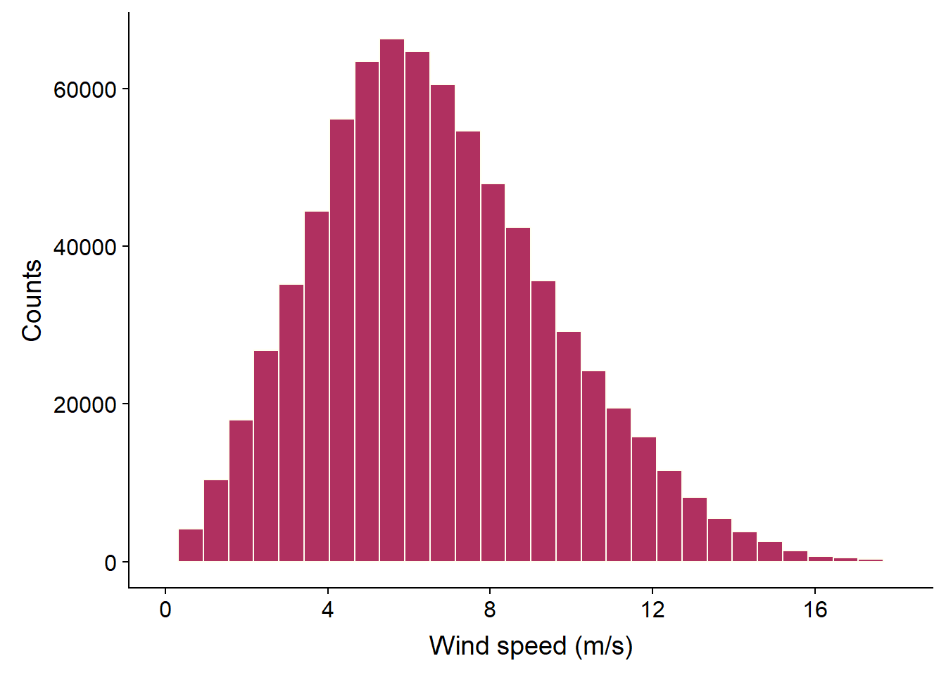
Figure 5: Distribution of weekly Wind speed recorded between January 1 to October 23, 2018 in the tropical Indina Ocean
# psych::describe(velocity.week$velocity)Figure 6 show daily wind speed of wind speed for 43 weeks in the tropical Indian Ocean region
wind.animate.week =  ggplot() +
  geom_raster(data = velocity.week,
              aes(x = longitude, y = latitude, fill = velocity), interpolate = FALSE)+
  geom_sf(data = spData::world, col = "black", fill = "ivory")+
  coord_sf(xlim = c(30,60), ylim =  c(-30,5))+
  scale_fill_gradientn(name = "Wind\nSpeed\n(m/s)", limits = c(0,15),
                       colours = oceColorsPalette(120), na.value = "White")+
  theme_bw()+
  theme(panel.background = element_rect(fill = "white"),
        axis.text = element_text(size = 11, colour = 1),
        panel.grid = element_line(colour = NA),
        legend.position = c(.1,.25),
        legend.background = element_rect(colour = NA, fill = "ivory"))+
  scale_x_continuous(breaks = c(35,55))+
  scale_y_continuous(breaks = c(-25, 2)) +
    labs(x = NULL, y = NULL)+
  #animate
  labs(title = 'Week: {frame_time}')+
  transition_time(week) +
  ease_aes('linear')

wind.animate.week
Figure 6: Animated of weekly Wind speed for 2018 in the tropical Indina Ocean
# you can control the speed of the animation with the animate() and parse argument fps =
# animate(wind.animate.week, fps = 2)
velocity.month = velocity.all %>%
group_by(longitude, latitude, month) %>%
summarise(velocity = mean(velocity, na.rm = TRUE))
velocity.month$month = as.integer(velocity.month$month)Figure 7 wind speed for the twelve ten months
## make label month

velocityMonth = velocity.month %>%
  mutate(day = 15, year = 2018, date = make_date(year, month, day),
         Month = month(date, abbr = FALSE, label = TRUE)) %>%
  select(date,month, Month, longitude, latitude, velocity)

  ggplot() +
  geom_raster(data = velocityMonth,
              aes(x = longitude, y = latitude, fill = velocity), interpolate = FALSE)+
  geom_sf(data = spData::world, col = "black", fill = "ivory")+
  coord_sf(xlim = c(30,60), ylim =  c(-30,5))+
  scale_fill_gradientn(name = "Wind\nSpeed\n(m/s)", limits = c(0,15),
                       colours = oceColorsPalette(120), na.value = "White")+
  theme_bw()+
  theme(panel.background = element_rect(fill = "white"),
        axis.text = element_text(size = 11, colour = 1),
        panel.grid = element_line(colour = NA),
        legend.position = "right",
        legend.background = element_rect(colour = NA, fill = NA),
        legend.key.height = unit(2.5, "lines"),
        legend.key.width = unit(1, "lines"))+
  scale_x_continuous(breaks = c(35,55))+
  scale_y_continuous(breaks = c(-25, 2)) +
  labs(x = NULL, y = NULL)+
  facet_wrap(~Month, nrow = 2)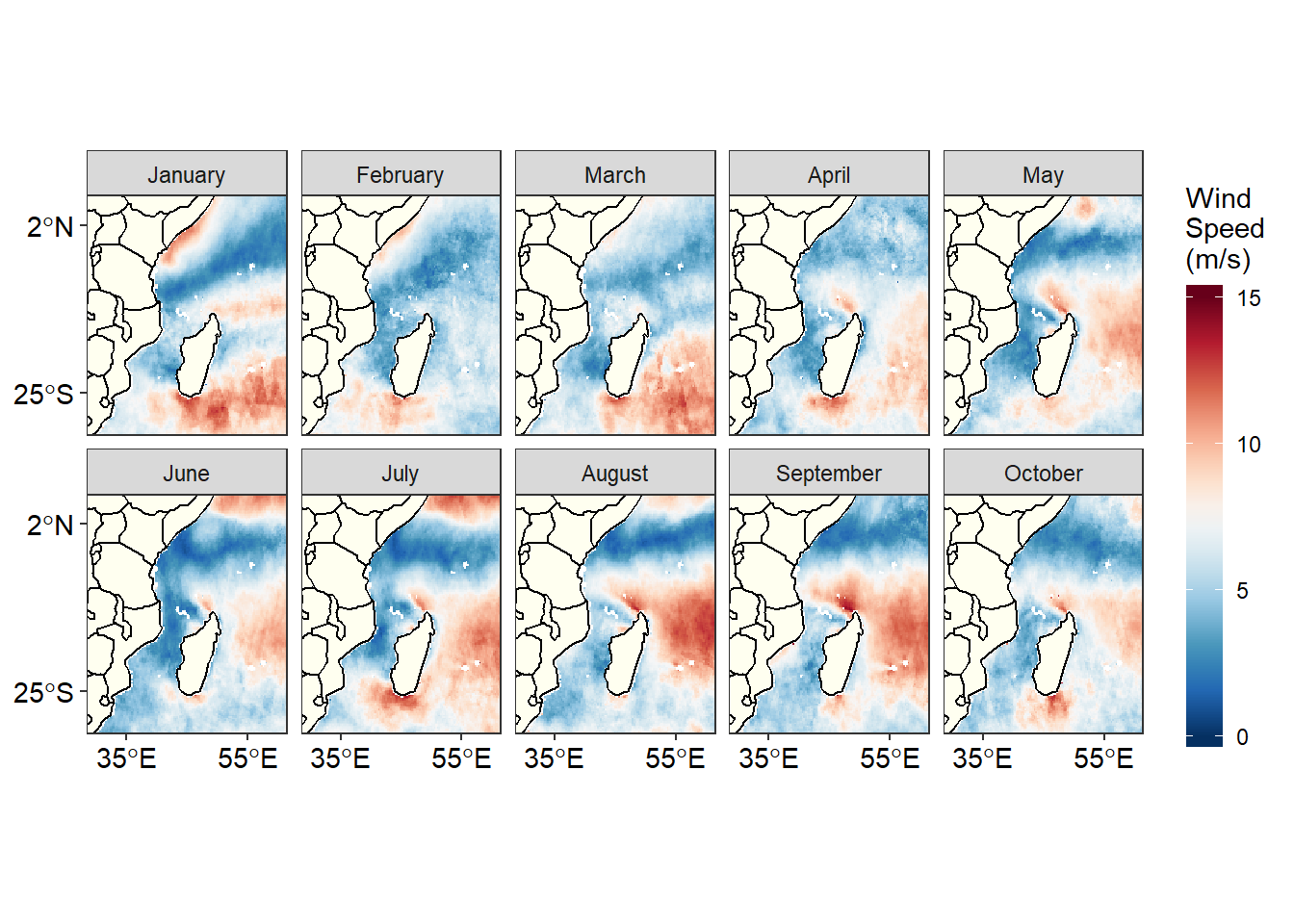
Figure 7: Map of the Tropical Indian Ocean showing monthly Wind speed for 2018
Figure 8 show minimum, maximum, median and outliers of wind speed for each month in the tropical Indian Ocean region
ggplot(data =velocityMonth %>% filter(between(velocity, 2,15) ),
       aes(x = Month, y = velocity, fill = as.factor(month)))+
  geom_boxplot(show.legend = FALSE)+
  scale_fill_brewer(palette = "Paired")+
  cowplot::theme_cowplot()+
  scale_y_continuous(breaks = seq(0,18,3))+
  scale_x_discrete(limits = month(seq(dmy(010118), dmy(301018), by = "month"),
      label = TRUE, abbr = FALSE) %>% rev())+
  coord_flip()+
  # labs(x = "", y = expression(~Wind~speed~(ms^{-1})))+ gganimate dont like expressions
  labs(y = "Wind speed (m/s)", x = "")+
  labs(title = "{closest_state}")+
  transition_states(month, transition_length = 5, state_length = 1, wrap = TRUE ) +
  ease_aes('linear') +
  shadow_mark()
Figure 8: Animate boxpot showing showing monthly Wind speed for 2018 in the Tropical Indian Ocean
Figure 9 is similar to 7, but Figure 9 is animated while figure 7 wind speed for the twelve ten months is static.
wind.animate.month = ggplot() +
  geom_raster(data = velocity.month,
              aes(x = longitude, y = latitude, fill = velocity), interpolate = FALSE)+
  geom_sf(data = spData::world, col = "black", fill = "ivory")+
  coord_sf(xlim = c(30,60), ylim =  c(-30,5))+
  scale_fill_gradientn(name = "Wind\nSpeed\n(m/s)", limits = c(0,15),
                       colours = oceColorsPalette(120), na.value = "White")+
  theme_bw()+
  theme(panel.background = element_rect(fill = "white"),
        axis.text = element_text(size = 11, colour = 1),
        panel.grid = element_line(colour = NA),
        legend.position = c(.1,.25),
        legend.background = element_rect(colour = NA, fill = "ivory"))+
  scale_x_continuous(breaks = c(35,55))+
  scale_y_continuous(breaks = c(-25, 2)) +
    labs(x = NULL, y = NULL) +
  labs(title = 'Month: {frame_time}')+
  transition_time(month) +
  ease_aes('linear')

wind.animate.month
Figure 9: Map of the Tropical Indian Ocean showing animated monthly Wind speed for 2018
quikscat
getInfo("qsux101day")
getInfo("qsuy101day")
Bibliography
Kelley, D., & Richards, C. (2018). Oce: Analysis of oceanographic data. Retrieved from https://CRAN.R-project.org/package=oce
Mendelssohn, R. (2018). Xtractomatic: Accessing environmental data from erd’s erddap server. Retrieved from https://CRAN.R-project.org/package=xtractomatic
R Core Team. (2018). R: A language and environment for statistical computing. Vienna, Austria: R Foundation for Statistical Computing. Retrieved from https://www.R-project.org/
Simons, R. (2011). ERDDAP–The environmental research division’s data access program.’. Available at Http. Coastwatch. Pfeg. Noaa. Gov/Erddap [2016].
Wickham, H. (2017). Tidyverse: Easily install and load the ’tidyverse’. Retrieved from https://CRAN.R-project.org/package=tidyverse
Wickham, H., François, R., Henry, L., & Müller, K. (2018). Dplyr: A grammar of data manipulation. Retrieved from https://CRAN.R-project.org/package=dplyr