ERDDAP is a web service developed by Bob Simons of NOAA serve a repository of environmental variables. There are over sixty ERDDAP servers providing access to a myriad satellite data and model output relevant to oceanography, meteorology, fisheries and marine mammals, among other areas. You find the dataset in this link https://coastwatch.pfeg.noaa.gov/erddap/metadata/fgdc/xml/. The good thing about ERDDAP is its ability to allow users define the area they interested and then subset data that is within the extent of the defined area.
Chamberlain (2017) developed rerddap package, which is a general purpose R client for working with ERDDAP servers within R environment. ERDDAP is a server built on top of OPenDAP, which serves some NOAA data. ERDDAP allow you to obtain data in either gridded or table format. rerddap has two main functions two download these two types. the griddap() lets you query from gridded datasets and tabledap() lets you query fom tabular dataset.
In this post I focus on getting geostrophic current of the Tropical Indian Ocean region from ERDDAP server using rerddap package in R environment (R Core Team, 2018). If you have the package in your machine you can proceed, but if not installed, you can install stable rerddap package from the cran or GitHub by uncomment the chunks below
#install.packages("rerddap")or development version from GitHub
#devtools::install_github("ropensci/rerddap")We call the rerddap package along with other package we will use for data processing and visualization with require() function.
require(rerddap)
require(sf)
require(tidyverse)
require(lubridate)
require(oce)
require(gganimate)
require(RColorBrewer)
A basemap was required that show the boundaries of the countries within the WIO region. The basemap that contain all African countries was used. Then load the basemap, for this post I used the basemap of Africa , which is the ESRI shapefile format. You can easily import shapefile into R workspace with the read_sf() function of sf package (Pebesma, 2018).
## read the shapefile
africa = read_sf("./africa/Spatial/AdmInfr/afcntry.shp")
To make labelling easy on map, I extracted the centroid location (longitude and latitude) from the polygons of country boundaries in Africa layer with st_centroid() and st_coordinates() function. The attribute information was extracted from the polgon geometry using expression st_geometry(country) = NULL. These attribute information was joined with centroid information with bind_col() function. Only the information for the countries within the tropical Indian Ocean region was retained and dropped information for other countries outside the region. Table 1 show the longitude and latitude and name of the countries in the western Indian Ocean region used to draw figure 1.
# extract centroid from polygones
centroids = africa%>%
  st_centroid() %>%
  st_coordinates() %>%
  as.tibble() %>%
  rename(lon = 1, lat = 2)

# make a copy of africa
country = africa

# remove the geometry and retain the attribute information of the africa countries
st_geometry(country) = NULL

# bind the country centroid information with the country attribute information
country.centroids = centroids %>%
  bind_cols(country) %>%
  # drop other variables except lon, lat and name
  select(lon,lat, name = CNTRY_NAME)

# select the countries in the wio region
country.wio = country.centroids %>%
  filter(name %in% c("Somalia", "Kenya", "Uganda", "Tanzania",
                     "Mozambique", "South Africa","Madagascar", "Comoros",
"Seychelles", "Mauritius", "Reunion"))| Longitude | Latitude | Country |
|---|---|---|
| 37.8618 | 0.5335 | Kenya |
| 46.7003 | -19.3793 | Madagascar |
| 35.5492 | -17.2637 | Mozambique |
| 57.5679 | -20.2869 | Mauritius |
| 55.5401 | -21.1208 | Reunion |
| 45.8673 | 6.0610 | Somalia |
| 55.5265 | -4.5965 | Seychelles |
| 34.8255 | -6.2655 | Tanzania |
| 32.3885 | 1.2816 | Uganda |
| 25.0800 | -28.9920 | South Africa |
| 43.6711 | -11.8875 | Comoros |
## draw map of the tropical indian ocean
ggplot() +
  geom_sf(data = spData::world, col = 1, fill = "ivory")+
  coord_sf(xlim = c(30,60), ylim = c(-30,5))+
  ggrepel::geom_text_repel(data = country.wio,
            aes(x = lon, y = lat, label = name), nudge_x = 0.05)+
  theme_bw() +
  theme(panel.background = element_rect(fill = "lightblue"),
        axis.text = element_text(size = 11, colour = 1),
        panel.grid = element_line(colour = NA))+
  scale_x_continuous(breaks = c(35,55))+
  scale_y_continuous(breaks = c(-25, 2)) +
  ggsn::scalebar(location = "bottomright", x.min = 35, x.max = 60,
                 y.min = -30, y.max = 5, dist = 600, dd2km = TRUE,
                 model = "WGS84", st.dist = 0.02, st.size = 4)+
  labs(x = NULL, y = NULL)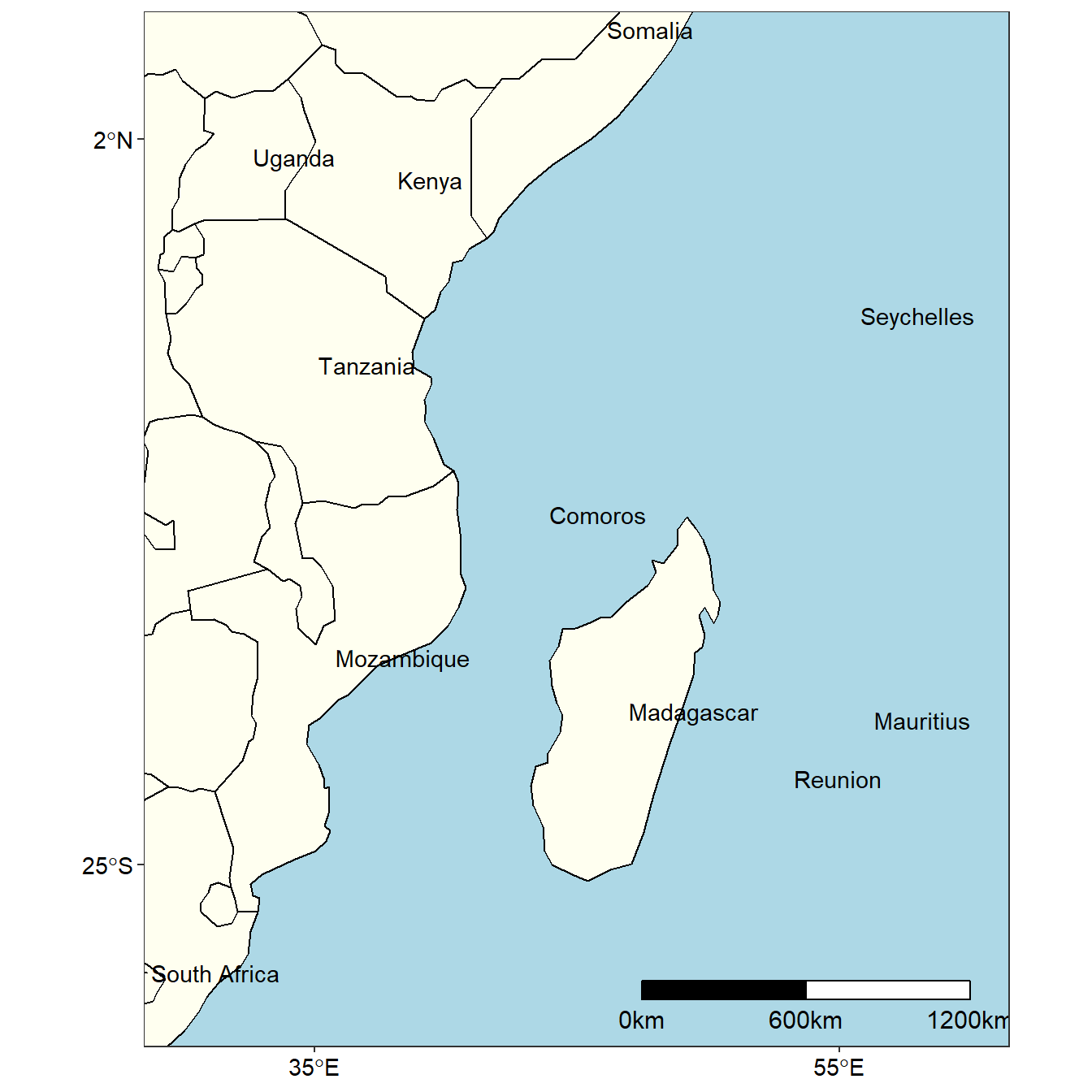
Figure 1: Countries in the western Indian Ocean region
Geostrophic Current
One main advantage of using ERDDAP is that you only need to download the subset of the data you desire, rather than the entire dataset. You can subset based on temporal— time range and spatial—geographical extent of interest. This approach is convinient and essential for oceanographic and environmental variables, which are usually large.
Aviso Zonal Geostrophic Current is inferred from Sea Surface Height Deviation, climatological dynamic height, and ba. I will download the AVISO geostrophic current from erdTAgeo1day_LonPM180 servers, which contain two gridded Variables:
- u_current (Eastward Sea Water Velocity, ms-1)
- v_current (Northward Sea Water Velocity, ms-1)
Since we know the datasetID is erdTAgeo1day_LonPM180 and unsure whether is gridded or tabular dataset, you can check the metadata of the dataset with rerddap function info().
## obtain metadata of the dataset
geoinfo = info("erdTAgeo1day_LonPM180")
geoinfo
<ERDDAP info> erdTAgeo1day_LonPM180
Dimensions (range):
time: (1992-10-14T12:00:00Z, 2012-12-08T12:00:00Z)
altitude: (0.0, 0.0)
latitude: (-90.0, 90.0)
longitude: (-179.7625173611111, 179.9875)
Variables:
u_current:
Units: m s-1
v_current:
Units: m s-1 If you do know the datasetId, the first way to find a dataset is to browse the builtin web page for a particular ERDDAP server. You can obtain a list of some public available ERDDAP servers with the servers() function as in the command below:
## call available ERDDAP servers
servers()
name
1 Marine Domain Awareness (MDA) - Italy
2 Marine Institute - Ireland
3 CoastWatch Caribbean/Gulf of Mexico Node
4 CoastWatch West Coast Node
5 NOAA IOOS CeNCOOS (Central and Northern California Ocean Observing System)
6 NOAA IOOS NERACOOS (Northeastern Regional Association of Coastal and Ocean Observing Systems)
7 NOAA IOOS NGDAC (National Glider Data Assembly Center)
8 NOAA IOOS PacIOOS (Pacific Islands Ocean Observing System) at the University of Hawaii (UH)
9 NOAA IOOS SECOORA (Southeast Coastal Ocean Observing Regional Association)
10 NOAA NCEI (National Centers for Environmental Information) / NCDDC
11 NOAA OSMC (Observing System Monitoring Center)
12 NOAA UAF (Unified Access Framework)
13 ONC (Ocean Networks Canada)
14 UC Davis BML (University of California at Davis, Bodega Marine Laboratory)
15 R.Tech Engineering
16 French Research Institute for the Exploitation of the Sea
url
1 https://bluehub.jrc.ec.europa.eu/erddap/
2 http://erddap.marine.ie/erddap/
3 http://cwcgom.aoml.noaa.gov/erddap/
4 https://coastwatch.pfeg.noaa.gov/erddap/
5 http://erddap.axiomalaska.com/erddap/
6 http://www.neracoos.org/erddap/
7 http://data.ioos.us/gliders/erddap/
8 http://oos.soest.hawaii.edu/erddap/
9 http://129.252.139.124/erddap/
10 http://ecowatch.ncddc.noaa.gov/erddap/
11 http://osmc.noaa.gov/erddap/
12 https://upwell.pfeg.noaa.gov/erddap/
13 http://dap.onc.uvic.ca/erddap/
14 http://bmlsc.ucdavis.edu:8080/erddap/
15 http://meteo.rtech.fr/erddap/
16 http://www.ifremer.fr/erddap/index.htmlSurface Geostrophic Currents From Altimetry
The geostrophic equations are widely used in oceanography to estimate currents. The basic idea is to use hydrographic measurements of temperature, salinity or conductivitiy, and pressure to calculate the density filed of the ocean using the equation of state of sea water. There are several satellite-altimeter systems measuring the oceanic geostrophic current. I will not cover them in this post.
Briefly Theory of Geostrophic
Satellite altimeters used to measure surface geostrophic currents also measure wave height. The geostrophic balance requires that the Coriolis force balance the horizontal pressure gradient. The equations for geographic balance are derived from the equations of motion assuming the flow has no accelaration, \(du/dt = dv/dt = dw/dt = 0\): that horizontal velocities are much larger than vertical, \(w < u,v\); that the only external force is gravity; and that friction is small. With these assumptions we obtain equation (1)
\[ \begin{align*} \frac{\delta p}{\delta x} = \rho f v \\ \frac{\delta p}{\delta x} = \rho f u \\ \frac{\delta p}{\delta x} = -\rho g \:\tag{1} \end{align*} \]
Where \(2\Omega sin \varphi\) is the Coriolis pparamer. The equation can be writen as equation (2)
\[ \begin{align*} u = \frac{1}{f \rho} \frac{\delta p}{\delta y}\\ v = \frac{1}{f \rho} \frac{\delta p}{\delta x} \tag{2} \end{align*} \]
The geostrophic approximation applied at \(z = 0\) leads to a very simple relation— surface geostrophic current are proportional to surface slope. For example, consider a level surface slightly below the se sea surface, say two meters below the sea surface , at \(z = -r\) equation (3)
\[ \begin{equation} u = v = w = 0 \tag{3} \end{equation} \]
The pressure of the level is obtained with equation (4)
\[ \begin{equation} p = \rho g\; (\zeta + r) \tag{4} \end{equation} \]
Assuming \(\rho\) and \(g\) are essentially constant in the upper few meters of the ocean. Sustituting this into equation (1) gives two components \(u_s, v_s\) of the surface geostrophic current writen in equation (5) The pressure of the level is
\[ \begin{align*} u_s = \frac{g}{f} \frac{\delta \varsigma}{\delta y}\\ v_s = \frac{g}{f} \frac{\delta \varsigma}{\delta x} \tag{5} \end{align*} \]
The Oceanic Topography
We can describe the topography of the sea surface \(\varsigma\) as the height of the sea surface relative to a particular level surface—the geoid. And geoid is the level surface that coincide with the surface of the ocean at rest. Thus, according to equation (eq:eq5) the surface geostrophic currents are proportional to the slope of the topography (figure 2)
cowplot::ggdraw() + cowplot::draw_image("geoid-01.png")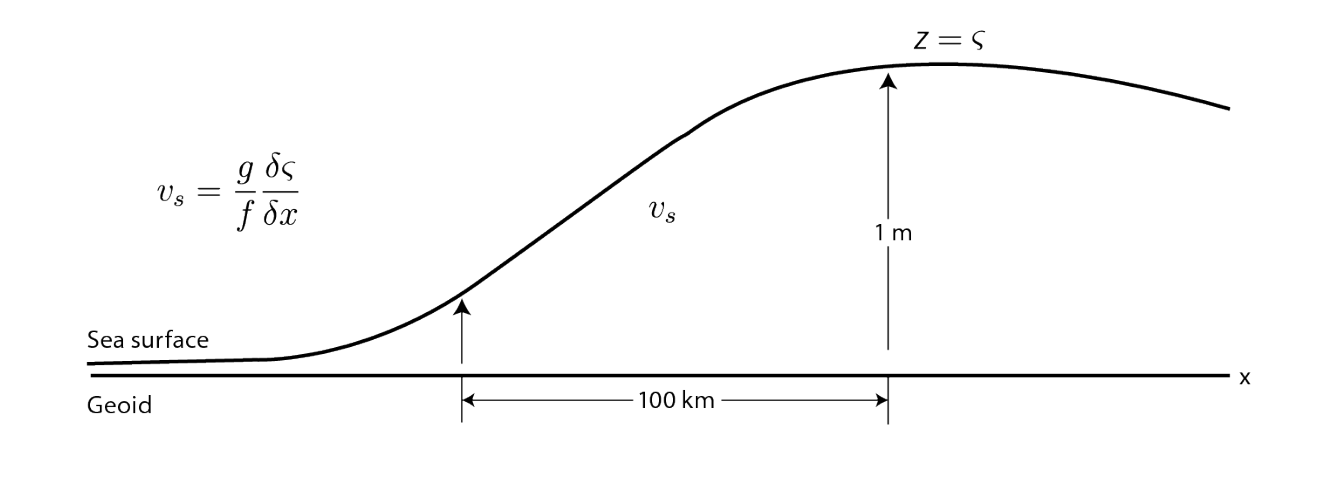
Figure 2: The slope of the sea surface relative to the geoid is direcltyl related to surface geostrophic currents. The slope of 1 meter per 100 kilometers is typical of strong currents
subsetting the Geostrophic Current
In the previous section I narrated a bit of the physics behind the geostrophic current. We now switch to AVISO that collects and process geostrophic currents from satellite. I first chopped the geostrophic current for the tropical Indian Ocean region with griddap() function. Like an R array, ERDDAP grids are subsetted by setting limits on the dimension variables, the difference being that a subset is defined in coordinate space (latitude values, longitude values, time values) rather than array space as is done with R arrays. Thus for erdTAgeo1day_LonPM180 the desired area of the data extract is latitude limits of (35 oS, 10 oN), longitude limits of (25 oE, 65 oE), and time limits of (1993-01-01, 2012-12-31) the following would be passed to the function griddap():
#get metadata information on an ERDDAP dataset
geoinfo = info("erdTAgeo1day_LonPM180")

## set spatial extent
lon = c(25,65)
lat =  c(-35,10)
## set temperal extent
time = c("1993-01-01", "2012-12-07")

## download the data
geostrophic = griddap(geoinfo, longitude = lon, latitude = lat,
                       time = time, fields = c("u_current", "v_current"))
Using equation (6) geostrophic current velocity was computed from the eastward (U) and northward (V) components of sea Water Velocity.
\[ \begin{equation} Velocity (ms^{-1})\:=\: \sqrt{(U^2+V^2)} \tag{6} \end{equation} \]
wio.geostrophic =  geostrophic %>%
  mutate(date = as.Date(time),
         vel = sqrt(u_current^2 + v_current^2)) %>%
  select(date, lon,lat, u = u_current, v = v_current, vel) %>%
  filter(date >= dmy(010112))
Table 2 show the sample of the geostrophic structure of the zonal (V) , meridional (U), current along the longitude and latitude and time within the tropical Indian Ocean region.
wio %>% sample_n(15) %>%
  kableExtra::kable("html", col.names = c("Date","Longitude", "Latitude", "Zonal (U)",
                                          "Meridional (V)","Velocity"),
                    align = "c", digits = 4,
                    caption = "wind data in the Western Indian Ocean Region")  %>%
  kableExtra::column_spec(column = 1:6, width = "8cm") %>%
kableExtra::add_header_above(c("", "Geographical Location" = 2, "Current Velocity" = 3))| Date | Longitude | Latitude | Zonal (U) | Meridional (V) | Velocity |
|---|---|---|---|---|---|
| 2012-08-13 | 53.2463 | 1.25 | -0.1657 | 0.0642 | 0.1777 |
| 2012-06-08 | 62.4957 | 0.50 | 0.0058 | -0.0016 | 0.0060 |
| 2012-11-01 | 51.9964 | 3.00 | -0.1440 | -0.0018 | 0.1441 |
| 2012-11-23 | 38.7473 | 3.00 | NA | NA | NA |
| 2012-10-18 | 58.2460 | -10.25 | -0.0179 | 0.0427 | 0.0463 |
| 2012-08-18 | 33.4977 | -32.25 | -0.0611 | 0.0193 | 0.0641 |
| 2012-06-16 | 55.4961 | -9.00 | 0.0000 | 0.0000 | 0.0000 |
| 2012-11-11 | 32.9977 | -18.50 | NA | NA | NA |
| 2012-07-19 | 37.2474 | -2.75 | NA | NA | NA |
| 2012-10-21 | 29.9979 | -22.50 | NA | NA | NA |
| 2012-05-21 | 63.2456 | 7.50 | -0.0480 | 0.0268 | 0.0550 |
| 2012-08-15 | 46.9967 | -20.50 | NA | NA | NA |
| 2012-05-24 | 46.7468 | 3.00 | -0.2065 | 0.2026 | 0.2893 |
| 2012-05-03 | 50.4965 | -33.50 | 0.0151 | -0.0002 | 0.0151 |
| 2012-07-03 | 38.2473 | -24.25 | -0.0021 | 0.0369 | 0.0370 |
Climatology geostrophic Current
To calculate the monthly climatology, the date variable in the dataset was separated into three variables—year, month and day using function from lubridate package (Grolemund & Wickham, 2011). Once the month variable were decomposed, the geostrophic values for each grid was grouped into months from January to December. Then the mean geostrophic value in the grid was calculated.
# decompose day, month, and year as separate variable from the date variable
wio = wio %>%
  mutate(day = day(date), month = month(date) %>%
           as.integer(), year = year(date)%>%
           as.integer())
## group current based on longitude, latitude and month
wio.month = wio %>% group_by(lon,lat,month) %>%
  summarise(u = mean(u, na.rm = T),v = mean(v, na.rm = T), vel= mean(vel, na.rm = T))

## ungroup grouped data frame
wio.month = wio.month %>% ungroup()
Table 2 shows climatological monthly ocean current dynamics in the tropical Indian Ocean region collected between 2012-01-04 and 2012-12-07. Figure 3 show the animated climatological monthly geostrophic current. The current velocity were mapped and animated with gganimate—grammar of animated graphics(Pedersen & Robinson, 2017) and ggplot2—grammar of graphics packages (Wickham, 2016)
ggplot() +
  geom_raster(data = wio.month,
              aes(x = lon, y = lat, fill = vel), interpolate = TRUE)+
  geom_sf(data = spData::world, col = 1, fill = "ivory")+
  coord_sf(xlim = c(30,60), ylim = c(-30,5))+
  # ggrepel::geom_text_repel(data = country.wio,
  #           aes(x = lon, y = lat, label = name), nudge_x = 0.05)+
  theme_bw() +
  theme(panel.background = element_rect(fill = "lightblue"),
        axis.text = element_text(size = 11, colour = 1),
        panel.grid = element_line(colour = NA),
        legend.key.height = unit(3, "lines"),
        legend.position = c(.92,.25),
        legend.background = element_rect(colour = 1))+
  scale_x_continuous(breaks = c(35,55))+
  scale_y_continuous(breaks = c(-25, 2)) +
  labs(x = NULL, y = NULL) +
  scale_fill_gradientn(colours = oceColors9A(120))+
  labs(title = 'Month: {frame_time}') +
  transition_time(month) +
  ease_aes('linear')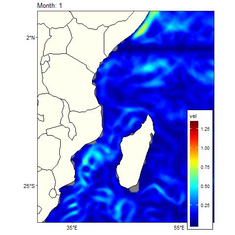
Figure 3: Climatology monthly mean Current in the tropical Indian Ocean region
Figure 4 show the animation of monthly climatological geostrophic current in the area around Somali current. We notice the area experience high speed geostrophic current above 0.5 ms-1 from June to October.
somali = wio.month %>% filter(lon < 53 & lat >2)

ggplot(data =somali ,
       aes(x = month, y = vel, fill = as.factor(month)))+
  geom_boxplot(show.legend = FALSE)+
  scale_fill_brewer(palette = "Paired")+
  cowplot::theme_cowplot()+
  scale_x_continuous(breaks = 1:12,
                     labels = month(seq(dmy(010118), dmy(311218), by = "month"),
                                    label = TRUE, abbr = TRUE))  +
  labs(title = "{closest_state}")+
  transition_states(month, transition_length = 5, state_length = 1, wrap = TRUE, states = ) +
  ease_aes('linear') +
  shadow_mark()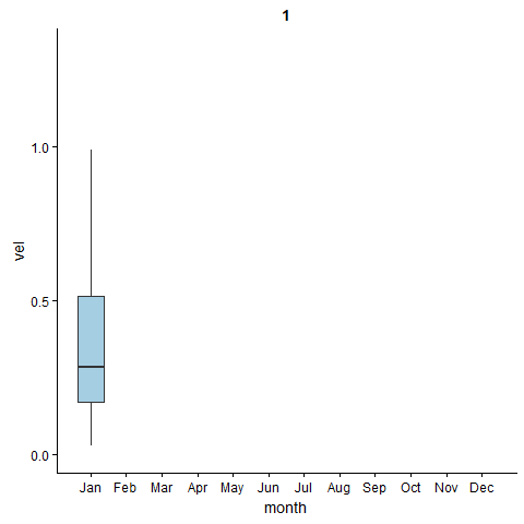
Figure 4: The monthly variation of geostrophic current in area around somali current
Remarks
The package rerddap has made access of oceanographic and environmental data into R. Once the data is in the workspace, we can transform, visualize and even animate to uncover subtle clue happening in the tropical Indian Ocean.
Literature
Chamberlain, S. (2017). Rerddap: General purpose client for ’erddap’ servers. Retrieved from https://CRAN.R-project.org/package=rerddap
Grolemund, G., & Wickham, H. (2011). Dates and times made easy with lubridate. Journal of Statistical Software, 40(3), 1–25. Retrieved from http://www.jstatsoft.org/v40/i03/
Pebesma, E. (2018). Sf: Simple features for r. Retrieved from https://CRAN.R-project.org/package=sf
Pedersen, T. L., & Robinson, D. (2017). Gganimate: A grammar of animated graphics. Retrieved from http://github.com/thomasp85/gganimate
R Core Team. (2018). R: A language and environment for statistical computing. Vienna, Austria: R Foundation for Statistical Computing. Retrieved from https://www.R-project.org/
Wickham, H. (2016). Ggplot2: Elegant graphics for data analysis. Springer-Verlag New York. Retrieved from http://ggplot2.org