Moving from ARGIS to R
For years, ESRI ArcGIS was a core software for most data processing, spatial analysis and drawing of outputs as map. Honestly the elegant high-resolution figures and maps I produced did not come from ArcMap, but rather from Adobe Illustrator. I was doing all the layout of the maps in ArcMap and then export it as in vector format Encapsulated PostScript. I then imported the .eps file into Adobe illustrator for touching and polishing. Although ArcMap has many cartographic tools and abilities (ArcGIS, 2011), but a lot of professional cartography is done in a vector graphics software such as Adobe Illustrator (and/or an image editing software such as Adobe Photoshop) (Adobe Illustrator, 2013) .
The main reason for using Adobe Illustrator was that it is a more robust graphics software package and provides tools and effects not available in ArcGIS. These allow me to access and manipulate each and every object on the page as a graphic object, even the individual vertices of the text letters. Therefore, combining ArcMap and Adobe Illustrator provided me the best I wanted. But the labour invested in creating a single graph or map was painful. Another main reason for looking for an alternative was the license issue. Esri Arcmap and Adobe Illustrator are proprietary software and hook your pocket for using them— unable to purchase the license for using the software in developing countries. The other reason made me sick of the combinantion is when I was asked to make some edits on the graphics or maps created. I hated to go back and redo the same procedures to make the same map and accomodate the correction. My mind frequently flushed with an idea to make the procedure to make map and graphics once and then reproduce it. However, that was far from the reality because ArcGIS and Adobe Illustrator are two different platform.
Coding with programming language was the solution to avoid repeatitive procedure to the common tasks. In 2015, I switched to R. One of the main reasons motivated me to invest my time and resources in R is it’s strong graphic power (R Core Team, 2018) and reproducibility. In this post I will explain and show how to make elegant map with standard quality even for publishing. We first need to load the packages we need for drawing maps.
require(tidyverse)
require(spData)
require(sf)
Importing and Processing Spatial Data
A basemap was required that show the boundaries of the countries within the WIO region. The basemap that contain all african countries was used. Then load the basemap, for this post I used the basemap of Africa , which is the ESRI shapefile format. You can easily import shapefile into R workspace with the read_sf() function of sf package (Pebesma, 2018).
## read the shapefile
africa = read_sf("./africa/Spatial/AdmInfr/afcntry.shp")
Because I was working with the Western Indian Ocean region, I chopped the four countries of interest and dump the rest of the polygons in the layer with filter() function from dplyr package (Wickham, François, Henry, & Müller, 2018). Trimming off unwanted polygons in a layer not only speed up drawing speed of the computer but also reduce processing time.
## read the shapefile
africa = read_sf("./africa/Spatial/AdmInfr/afcntry.shp")

## seclect the countries of Tanzania, Kenya and Mozambique nad Madagascar
wio = africa%>%
  select(-c(FIPS_CNTRY, REGIONA, EMPTY, EMPTY2))%>%
  filter(CNTRY_NAME == "Tanzania" |
           CNTRY_NAME == "Kenya" |
           CNTRY_NAME == "Mozambique" |
           CNTRY_NAME == "Madagascar")
Once the African boundary shapefile was filtered too obtain the three boundaries of Kenya, Tanzania, Mozambique and Madagascar where the sampling was done. The geographical location of the sampling station was also ingested in R’s worksapace. Since the file was in Excel spreashead, the read_excel() function from readxl package was used to import the file (Wickham & Bryan, 2018)
# stations
point = readxl::read_excel("./Ogalo_mgeleka/stations.xlsx")
Once the file was in the workspace, it was tied—cleaned and structured in a way make analysis and plotting easy. To make the data tidy and avoid clusters of points, only a single station was retained for areas with more than one station (Table 1)
point.select = point  %>%
  filter(Site %in% c("Inhaca South", "Inhaca North", "Nosy Beach East", "
                     Pemba", "Mbweni"))

point.select=point.select %>%
  mutate(Site = replace(Site,Site == "Mbweni", "Zanzibar"),
         Site = replace(Site,Site == "Nosy Beach East", "Nosy Beach"))

point %>% kableExtra::kable("html", caption = "Geographical positions of the stations",
                col.names = c("Stations", "Longitude", "Latitude"), digits = 4, align = "c") %>%
  kableExtra::column_spec(column = 1:3, color = 1, width = "4cm") %>%
kableExtra::add_header_above(c("", "Geographical Locations" =2), align = "c")| Stations | Longitude | Latitude |
|---|---|---|
| Inhaca South | -26.0356 | 32.9323 |
| Inhaca North | -25.8287 | 32.9139 |
| Pemba | -12.9678 | 40.5474 |
| Fumba | -6.3224 | 39.2890 |
| Mbweni | -6.2238 | 39.1970 |
| Chwaka | -6.1623 | 39.4414 |
| Nungwi | -5.7173 | 39.3019 |
| Mjimwema | -6.8231 | 39.3500 |
| Mombasa | -4.0115 | 39.7287 |
| Nosy Beach East | -13.5179 | 48.4650 |
| Nosy Beach West | -13.5233 | 48.4256 |
Then the tidy was converted from tabular formaat to simple feature—equvaivalent to popular spatial format shapefile. The transformation of tabular to shapefile was done using the combination of function from the sf package
point.sf = point %>%
  st_as_sf(coords = c("Long", "Lat")) %>%
  st_set_crs(4326)
Mapping
Once the data was cleaned and converted to the right format, a ggplot2 was used to create graphic.geom_sf() was used to draw maps the simple feature objects and limit the areas with coord_sf(). geom_label_repel() function from ggrepel package was used to label the sampling stations and the scalebar() function from ggsn package was used to draw scale on map. After the tweeking of different geom and them I ended up with map in figure 1
wio.map = ggplot() +
  geom_sf(data = spData::world, col = 1, fill = "ivory")+
  coord_sf(xlim = c(30,60), ylim = c(-30,5)) +
  geom_point(data = point.select, aes(x = Long, y = Lat), size = 2)+
  ggrepel::geom_text_repel(data = point.select, aes(x = Long, y = Lat, label = Site), nudge_y = 1.5, nudge_x = 5)+
  theme_bw() +
  theme(panel.background = element_rect(fill = "lightblue"),
        axis.text = element_text(size = 11, colour = 1),
        panel.grid = element_line(colour = NA))+
  scale_x_continuous(breaks = c(35,55))+
  scale_y_continuous(breaks = c(-25, 2)) +
  ggsn::scalebar(location = "bottomleft", x.min = 35, x.max = 60,
                 y.min = -30, y.max = 5, dist = 600, dd2km = TRUE,
                 model = "WGS84", st.dist = 0.02, st.size = 4)+
  labs(x = NULL, y = NULL)


wio.map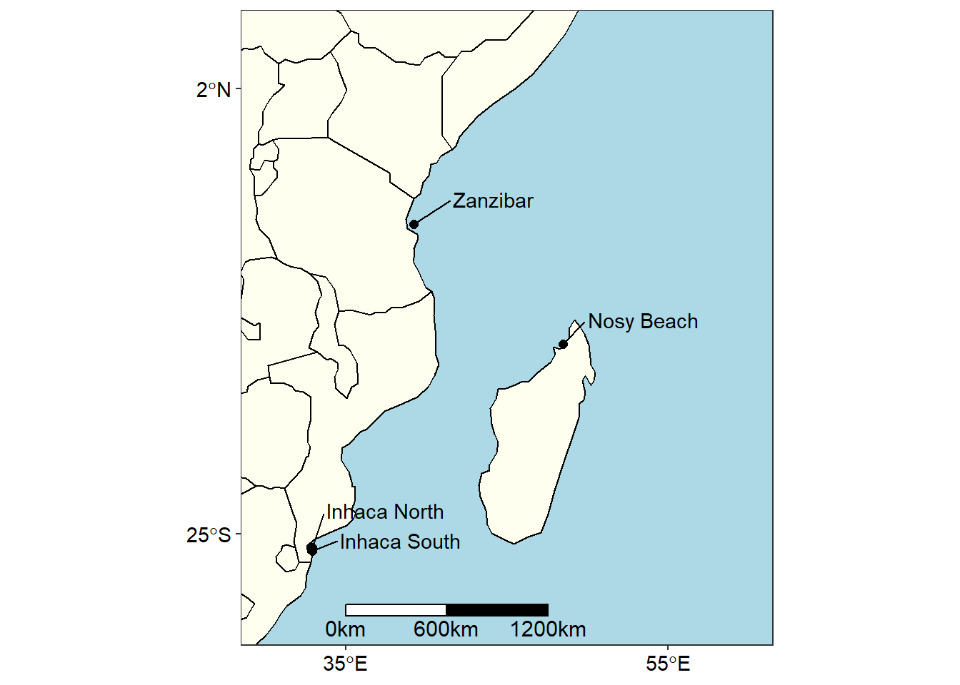
Figure 1: map
Though figure 1 show the sampling areas within the Western Indian Ocean Region, its large scale masked subtle information of sampling station in these areas. For example, with figure 1 we are able to show just a location in Zanzibar, but there were four sampling station in this area as revealed in zoomed portion of the island in figure 2
zanzibar =ggplot()+
  geom_sf(data = wio, col = "black", fill = "ivory")+
  coord_sf(xlim = c(38.825, 39.6), ylim = c(-6.5, -5.63785)) +
  geom_point(data = point,
  aes(x = Long, y = Lat), size = 2)+
  ggrepel::geom_text_repel(data = point  %>%
  filter(Site %in% c("Nungwi", "Chwaka", "Fumba", "Mbweni")),
  aes(x = Long, y = Lat, label = Site), point.padding = 0.2, nudge_y = 0.005,
  nudge_x = -0.12, segment.colour = "red", direction = "y")+
  theme_bw() +
  theme(axis.text = element_text(size = 11, colour = 1),
        panel.background = element_rect(fill = "lightblue"),axis.title = element_blank(),
        panel.grid = element_line(colour = NA))+
  # scale_x_continuous(breaks = c(36.10, 39.55))+
  scale_y_continuous(breaks = c(-6.4, -5.7))+
  scale_x_continuous(breaks = c(38.9, 39.5))


zanzibar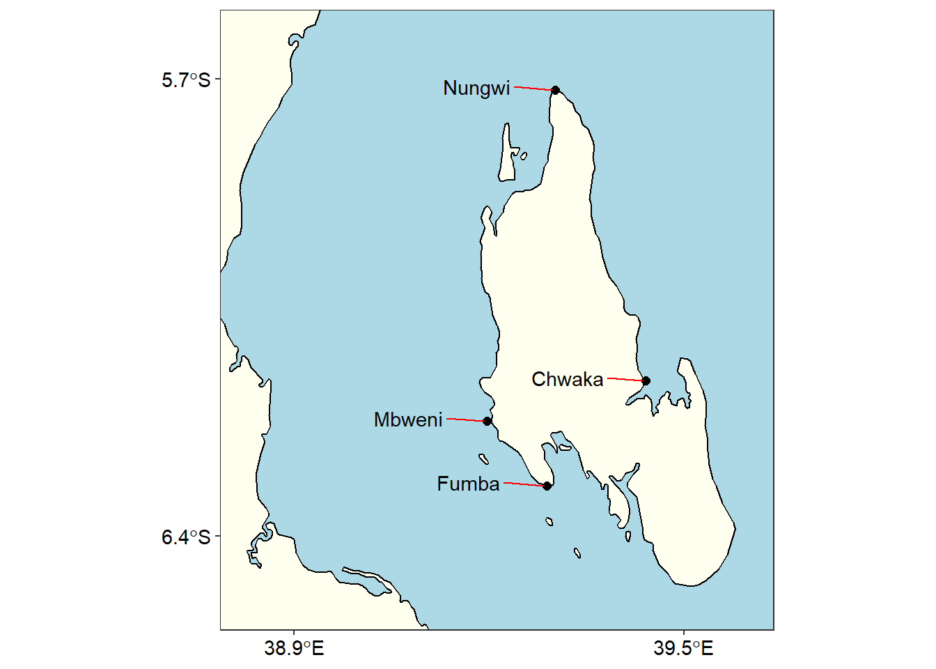
Figure 2: Sampling stations at Unguja Island
Similar to Unguja, there were two stations at Madagascar, but in figure 1 they clustered because of the small scale used and becomes difficult to present them on the map. However, when we use a large scale, we obtain a much clear graphic of the area (Figure 3)
nosy = ggplot()+
  geom_sf(data = wio, col = "black", fill = "ivory")+
  coord_sf(xlim = c(48.38, 48.5), ylim = c(-13.58, -13.48)) +
  geom_point(data = point,
  aes(x = Long, y = Lat), size = 4)+
  ggrepel::geom_text_repel(data = point  %>%
  filter(Site %in% c("Nosy Beach East", "Nosy Beach West")),
  aes(x = Long, y = Lat, label = Site), point.padding = 0.2, nudge_y = .0025, nudge_x = -0.03, segment.colour = "red")+
  theme_bw() +
  theme(axis.text = element_text(size = 11, colour = 1),
      panel.background = element_rect(fill = "lightblue"),axis.title = element_blank(),
      panel.grid = element_line(colour = NA))+
  scale_x_continuous(breaks = c(48.39, 48.49))+
  scale_y_continuous(breaks = c(-13.57, -13.49))

nosy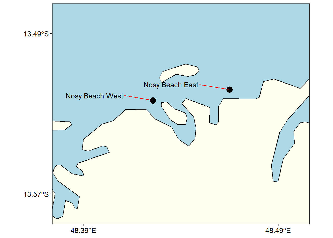
Figure 3: Sampling stations at Nosy Madagascar
Further, there were two sampling points at Inhaca that are not visible in figure 1.Zooming in at the location the distance between the points were clearly visible as shown in figure 4
inhaca = ggplot()+
  geom_sf(data = wio, col = "black", fill = "ivory")+
  coord_sf(xlim = c(32.4, 33.17), ylim = c(-26.4,-25.62)) +
  geom_point(data = point,  aes(x = Long, y = Lat), size = 4)+
  geom_text(data = point, aes(x = Long, y = Lat, label = Site), nudge_x = -0.05, nudge_y = 0.05, size = 4.2)+
  theme_bw() +
  theme(axis.text = element_text(size = 11, colour = 1),
      panel.background = element_rect(fill = "lightblue"),axis.title = element_blank(),
      panel.grid = element_line(colour = NA)) +
  scale_x_continuous(breaks = c(32.5, 33.1))+
  scale_y_continuous(breaks = c(-26.3, -25.7))

inhaca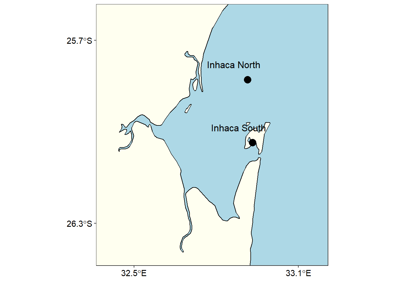
Figure 4: Sampling stations at Inhaca Mozambique
Wilke (2018) developed a cowplot package which has tools to combine figures. For example the chunk below was used to combine figure 5
cowplot::plot_grid(zanzibar, inhaca, nrow = 1, labels = c("A", "B"),
                   label_x = .16, label_y = .85, label_fontface = )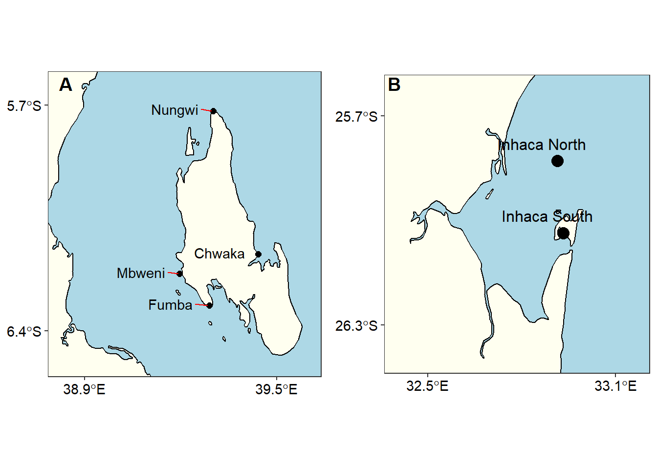
Figure 5: The stations in A) Unguja-Tanzania and B) inhaca - Mozambique
with cowplot package , it is possible to place several inset maps on the main map using the ggdraw() and draw_plo() functions. For example the chunk below produce the figure 6.
cowplot::ggdraw()+
  cowplot::draw_plot(wio.map, x = 0, y = 0, width = 1, height = 1)+
  cowplot::draw_plot(nosy+theme(axis.text = element_blank(), axis.ticks = element_blank()),
                     x = .51, y = 0.2,width = .6, height = .6,scale = .5)+
  cowplot::draw_plot(zanzibar+theme(axis.text = element_blank(), axis.ticks = element_blank()),
                     x = .4, y = 0.49,width = .6, height = .6,scale = .6)+
  cowplot::draw_plot(inhaca+theme(axis.text = element_blank(), axis.ticks = element_blank()),
                     x = .41, y = -0.05,width = .6, height = .6,scale = .6)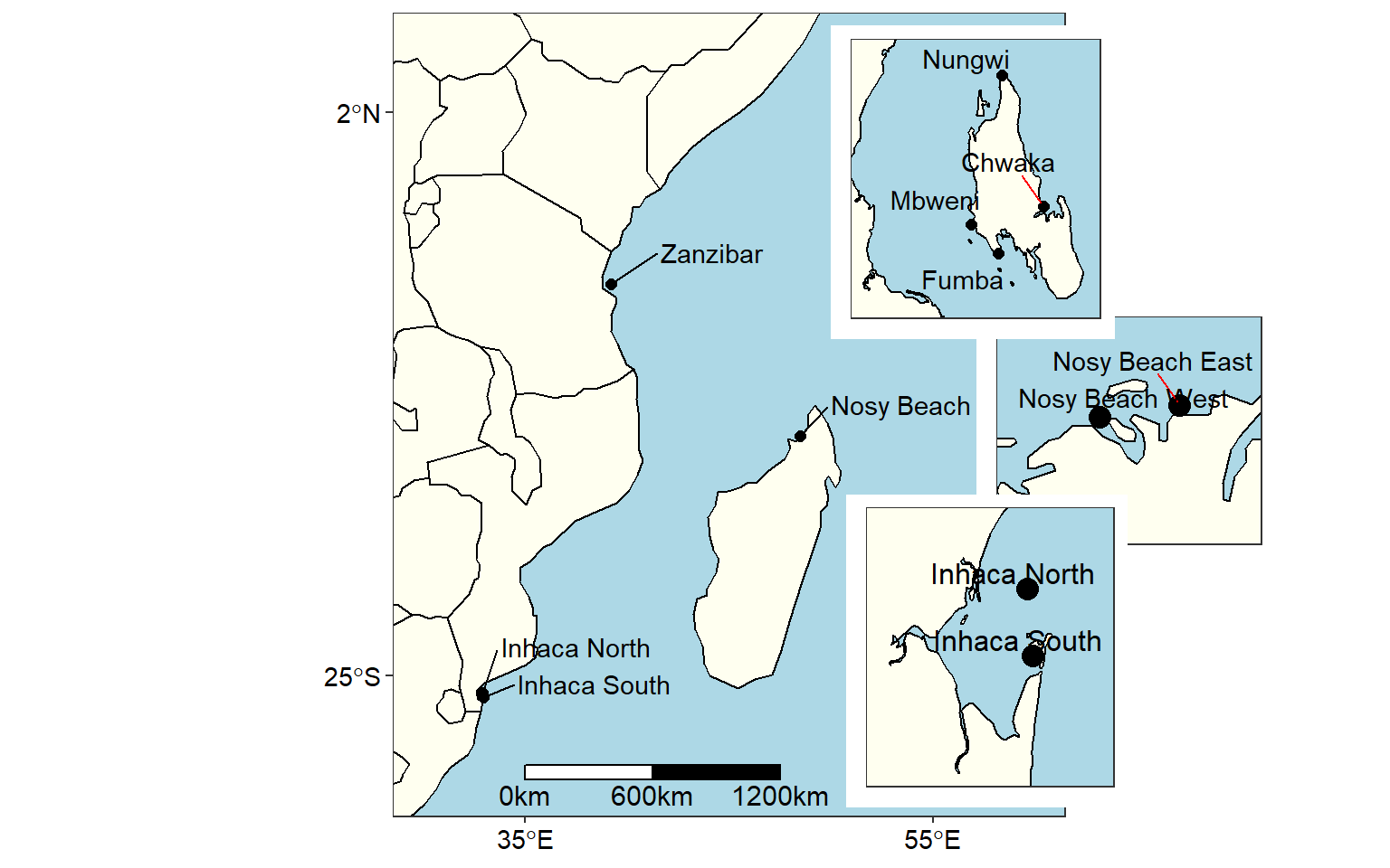
Figure 6: Map of area of interest drawn on on the WIO region area to show sampling stations
Conclusion
We have seen the power of R and ggplot2 to draw the publication quality graphics. With cowplot package, we can combine several graphics in a single layout. I have note done with Adobe illustrator—is still in high rank of software in my softwarebox. I still use this powerful software to edit and polish vector graphics generated from R like in figure7. The dotted line in figure7 are ocean current in the Western Indian Ocean region. The map was done in R, exported as .eps and ocean current—dotted line were drawn in adobe illustrator environement.
cowplot::ggdraw() +
  cowplot::draw_image("map.png" )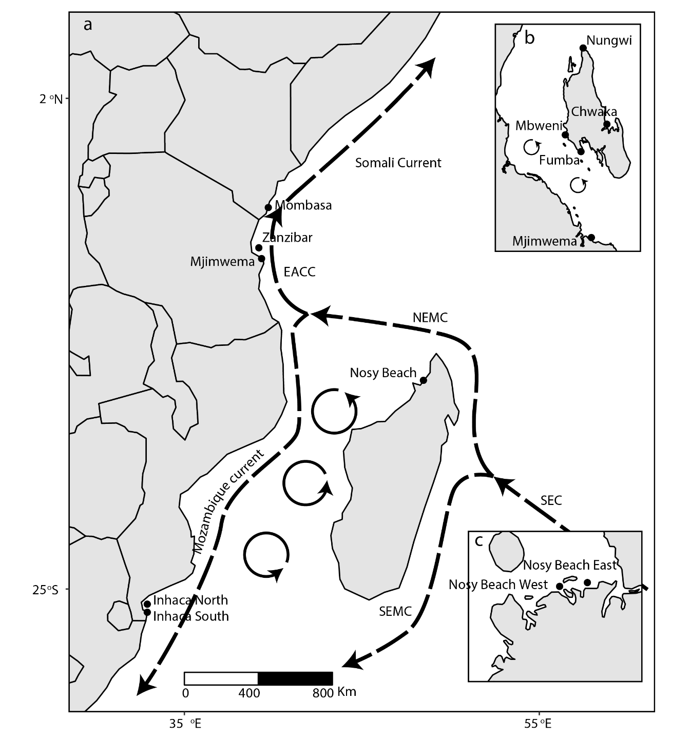
Figure 7: Ocean current in the WIO region
Bibliography
Adobe Illustrator, C. (2013). Classroom in a book–Adobe creative team. Peachpit Press.
ArcGIS, E. (2011). Release 10. Redlands, CA: Environmental Systems Research Institute, 437, 438.
Pebesma, E. (2018). Sf: Simple features for r. Retrieved from https://CRAN.R-project.org/package=sf
R Core Team. (2018). R: A language and environment for statistical computing. Vienna, Austria: R Foundation for Statistical Computing. Retrieved from https://www.R-project.org/
Wickham, H., & Bryan, J. (2018). Readxl: Read excel files. Retrieved from https://CRAN.R-project.org/package=readxl
Wickham, H., François, R., Henry, L., & Müller, K. (2018). Dplyr: A grammar of data manipulation. Retrieved from https://CRAN.R-project.org/package=dplyr
Wilke, C. O. (2018). Cowplot: Streamlined plot theme and plot annotations for ’ggplot2’. Retrieved from https://CRAN.R-project.org/package=cowplot