Packages
We need some packages to process ADCP data. These packages includes
require(oce)
require(tidyverse)
require(visdat)
require(naniar)
require(UpSetR)
Ingest the ADCP
The LTA dataset was imported into R with read.adp() function from oce package
pemba = read.adp("./adcp/ADCP_DATA/2007_05/M72-5_OS75011_000000.LTA")Extract variables contained
The ADCP was collected using the broadband instrument with a frequency of 75KHz making a total of 100 cells spaced at an interval of 16 m making a profile of 1600 m deep. The instrument was configured with four beams, each beam measure the meridional-east (V), zonal-north (U) components, the the up and error.
#summary(pemba)

beamName(pemba)
## [1] "east" "north" "up" "error"east = pemba[["v"]][,,1]
north = pemba[["v"]][,,2]
distance = pemba[["distance"]]
time = pemba[["firstTime"]]
ship.speed = pemba[["avgSpeed"]]
lon = pemba[["firstLongitude"]]
lat = pemba[["firstLatitude"]]Transforming
calculate velocity from the northe and south components and then create a data frame from this components.
vel = sqrt(east^2 + north^2)

dt = data.frame(distance, vel)
Visualize
Figure 1a show the vertical profile of current velocity measured at the station. Although the profile showed the full length from the surface to 1600 m, we noticed that the actual value reached a maximum depth of 250 m (Figure 1b). Beyond this depth there was no current data (Figure 1a).About 86 percent of cells have missing values compared to 14 percent of cell with current velocity (figure 2).
cowplot::plot_grid(fig1a,fig1b, nrow = 1,
                   labels = c("a)", "b)"),
                   label_size = 14,
                   label_fontface = "plain",
                   label_x = 0.2, label_y = .85)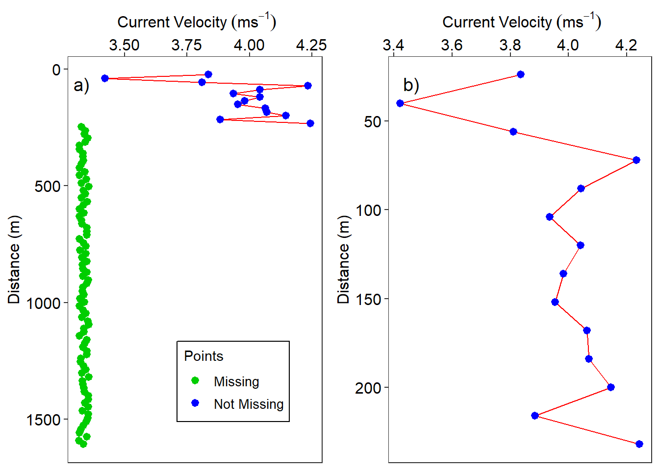
Figure 1: Current profiles a)
vis_miss(dt%>%select(vel))+
  theme(axis.text = element_text(colour = 1, size = 12),
        legend.text = element_text(size = 11, colour = 1),
        legend.position = c(.86,.25),
        legend.background = element_rect(colour = 1, fill = "white"))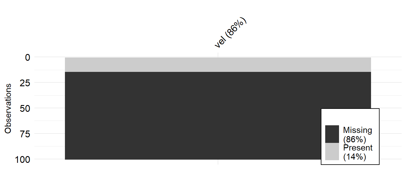
Figure 2: The Percentage of missing values in the profile