Introduction
The OpenFisheries.org project created an open web platform aimed to advance the practice of data science in fisheries. The project has managed to consolidate global fisheries dataset that can be accessed and retrieved using modern analytics. The OpenFisheries.org flagship project is the Global Fisheries REST API forms the backbone of fisheries data science, enabling reproducible analytics in R (R Core Team, 2019), Python or any other language.
The capture fisheries data for OpenFisheries landings API comes from the UN Food and Agriculture Organization. Karthik Ram, Carl Boettiger and Andrew Dyck developed rfisheries package (Ram et al., 2016) that allows anyone familiar with R programming access FAO’s Fisheries and Aquaculture statistics. As I was writing this post, the package can only retrieve capture annual fish landing catches from 1950-2015. In this post I illustrate how to use the rfisheries package to get fisheries data. This can be useful, especially for anyone interested with comparing capture fisheries from multiple countries over a certain period.
To make use of functions available in the rfisheries package, we need to load it into the workspace. This is possible if the package has already installed in the machine. Otherwise we need to install the development version of the package as shown in the code below;
if (!require("devtools")) install.packages("devtools")
devtools::install_github("ropensci/rfisheries")
We then load the packages that we use to access the data, manipulate and visualize the results. The rfisheries interact with the API and fetch the data based on the query provided. The tidyverse contains packages that help us to manipulate, analyse and even visualize the fisheries statistics in a consistency manner (Wickham, 2017).
require(tidyverse)
require(rfisheries)
Global Total Fisheries landing
Fisheries landings can be obtained with of_landings() function. Without parsing argument in the function, the results is the time series of annual total catches that span from 1950 to the up to date. The chunk below show the code that extracted global annual catch of capture fisheries reported.
annual.landings = rfisheries::of_landings()I have trimmed the data frame to show only the first and last five rows (Table 1)
| 1950 | 1951 | 1952 | 1953 | 1954 | 2011 | 2012 | 2013 | 2014 | 2015 |
|---|---|---|---|---|---|---|---|---|---|
| 19727413 | 22322503 | 23992129 | 24280658 | 26255749 | 92459929 | 89784576 | 91588095 | 92030328 | 92588168 |
We can visualize tha pattern of capture fisheries over time. Figure 1 clearly indicate that the landing from capture fisheries has been increasing exponentially from less than 30MT in 1950 to over 90 MT in 1990 and since then the annual catches slightly oscilate around that 90MT
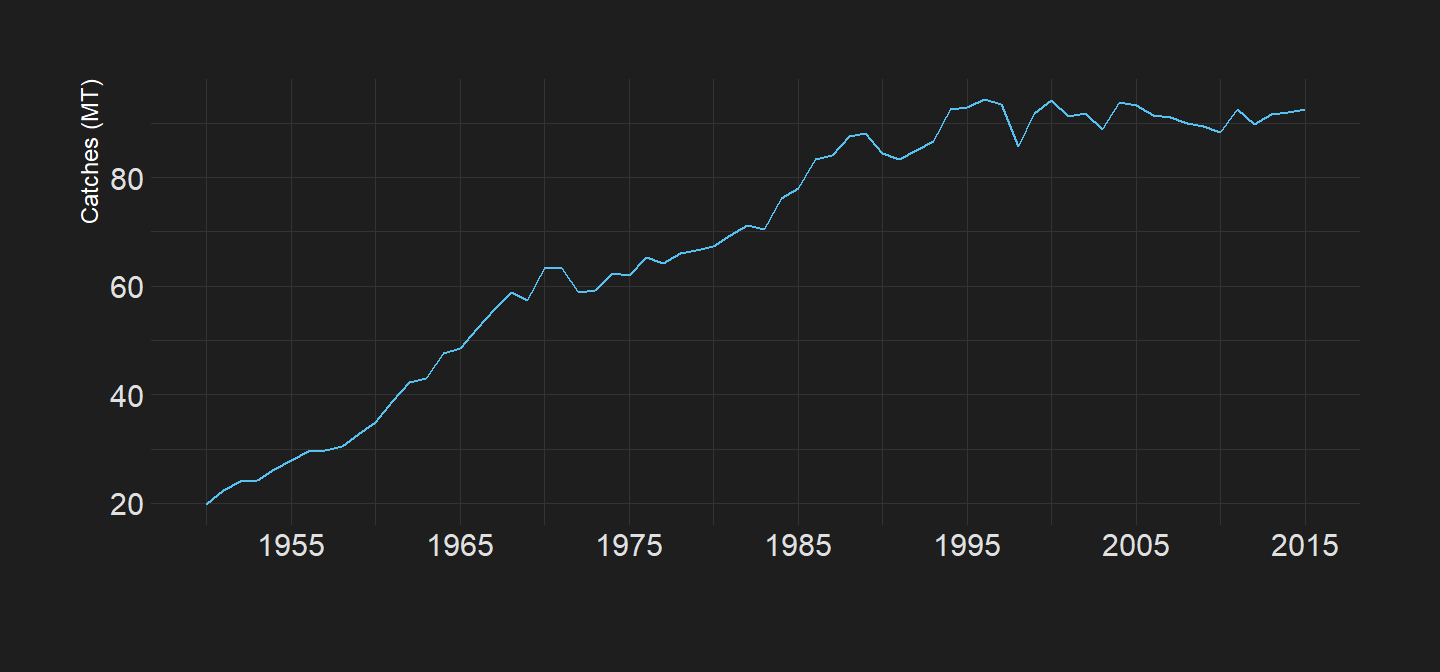
Figure 1: Global Annual Total Capture Fisheries Catches
Country’s Total Landings
Sometimes global landings may not suit the questions you want to answer, for instance you may be interested to compare the annual totat catches for multiple countries. To obtain the catches for a country of interest you must specify the argument country. Be aware that only the iso3c is accepted. the iso3c codes are three-letter that identify and represent represent countries, dependent territories, and special areas of geographical interest. If you cant figure out the country code, you can simply run `of_country_codes()’ to obtain the list of countries with their respective codes.
coundry.codes = of_country_codes()A list of ten sampled International Organization for Standardization (ISO) codes are shown in table 2
| Country | code |
|---|---|
| Albania | ALB |
| St. Pierre and Miquelon | SPM |
| Nigeria | NGA |
| Bahamas | BHS |
| Luxembourg | LUX |
| South Africa | ZAF |
| Lao People’s Dem. Rep. | LAO |
| Falkland Is.(Malvinas) | FLK |
| Côte d’Ivoire | CIV |
| Cape Verde | CPV |
Once we know the codes we can fetch the annual landing catches for the country of interest, for instance, we are interested to obtain the annual catches landed over the available period. the chunk below highlight the code that was used to access the total catches in Tanzania shown in figure 2.
annual.landings.tza = rfisheries::of_landings(country = "TZA")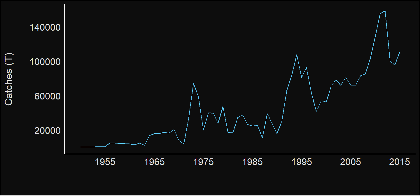
Figure 2: Annual capture fish landing in Tanzania Mainland
Landings from multiple countries.
Our interest is to compare the total landings from the WIO region, unfortunate, the of_landings() function does not allow us to query more than one at a time. To overcome this package limitation, we have to expand the process with other function available in R. And because the landing search is based on the country code, we first create a tibble that has a country code and their corresponding names (Müller and Wickham, 2018)
wio.countries = tibble(code = c("KEN", "TZA", "EAZ", "SYC", "ZAF", "MOZ",
                                "SOM", "MUS", "MYT", "MDG"),
                       name = c("Kenya", "Tanzania", "Zanzibar", "Seychelles",
                                "South Africa",   "Mozambique", "Somalia",
                                "Mauritius", "Mayotte", "Madagascar"))
We then iterate the process that search and download the landing of each country as the data. To chain the process, we make a landings.wio.list as a container that will store the download files. This is important because each iteration feeds into this list file. If you are unfamiliar with looping in R, please consult the relevant resources that guides on how you can use for loop to iterate processes.
landings.wio.list = list()

for (catches in 1:nrow(wio.countries)){
  landings.wio.list[[catches]] = rfisheries::of_landings(country = wio.countries$code[catches]) %>%
    rename(code = country) %>%
    mutate(name = wio.countries$name[catches])
}
The loop output a list files with multiple data frames of total catches for each country selected in the region. To expand our analysis and visualize the catch, we need to make a single data frame that contains all countries’ total landing from a list file. dplyr package has a nifty bind_row() function that does the work (Wickham et al., 2018) with a single line of code highlighted below;
landings.wio.tb = landings.wio.list %>% bind_rows()Once we have the data in the right format, we can visualize. The first I wanted to understand is how the catches varied among these countries in 2015 as seen. With few lines of code I was able to understand that Somalia reported the least catch and South Africa nailed the list with the highest catch in 2015 (Table 3). Here is the code that generated table 3.
| Year | Catch | Code | Country |
|---|---|---|---|
| 1969 | 800 | MYT | Mayotte |
| 1976 | 5477 | MYT | Mayotte |
| 1960 | 9366 | EAZ | Zanzibar |
| 1968 | 16578 | TZA | Tanzania |
| 1984 | 17251 | MYT | Mayotte |
| 1955 | 47183 | SYC | Seychelles |
| 1960 | 62832 | SYC | Seychelles |
| 2002 | 68134 | MDG | Madagascar |
| 2003 | 326993 | SYC | Seychelles |
| 1992 | 3878960 | ZAF | South Africa |
Comparing catches of all countries over the period , We notice that the higher catch landings from South Africa masks catches from other countries in the region (Figure 3).
 ggplot() +
  geom_line(data = landings.wio.tb,
            aes(x = year, y = catch/1000, col = name))+
  labs(x = "", y = "Catches (T)")+
  # theme(panel.grid.minor = element_blank(), legend.key = element_blank())+
  # scale_y_continuous(limits = c(0,100), breaks = seq(10,100,20))+
  scale_x_continuous(breaks = seq(1955,2015,20))+
  # scale_color_discrete(name = "Countries")+
  see::scale_color_material_d(name = "Countries")+
  see::theme_blackboard()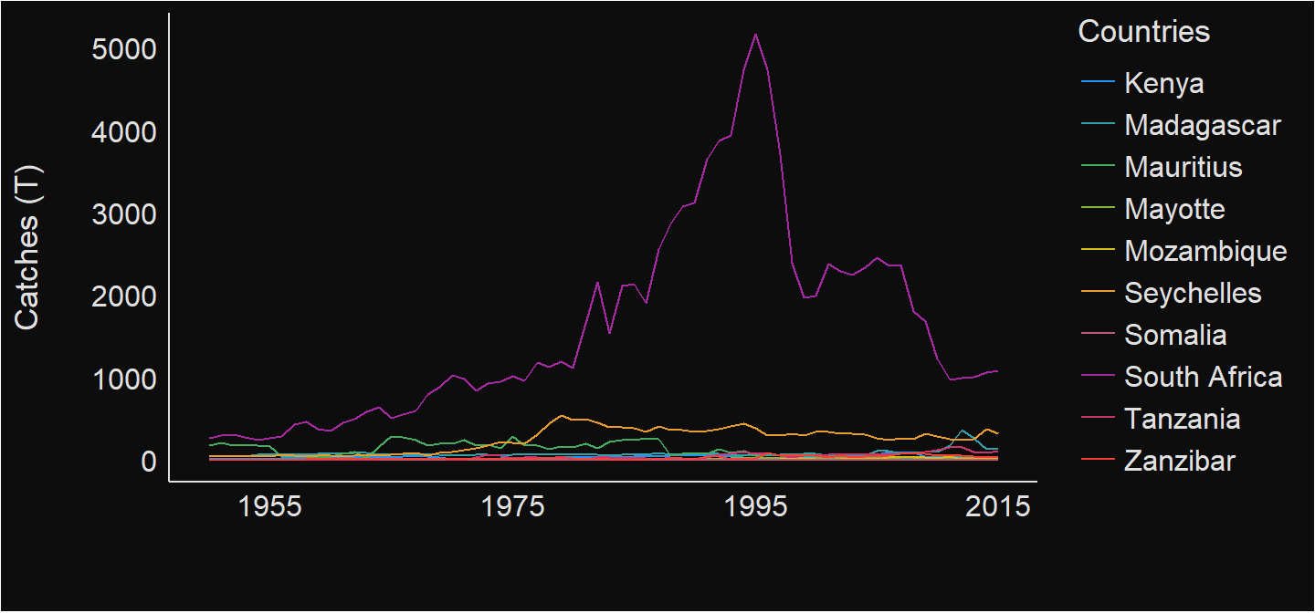
Figure 3: Annual total catch of ten selected countries in the WIO region
To make the plot visible and standout for each country, I decided to switch to multiple plots and make the landing scale free for each country. This make it easier to see the trends of fisheries landings separately for each country (Figure 4)
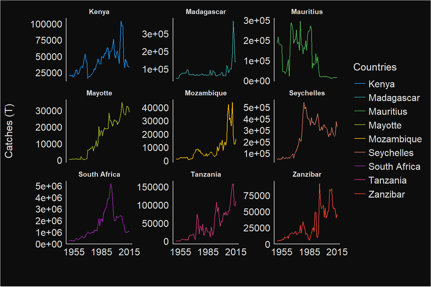
Figure 4: WIO region Capture Fisheries
I notice that the landing pattern differs from each country. While all other countries shows a dwindling trends, of interest is the increasing positive trend of landings in Mayotte (Figure 4). South Africa, Madagascar and Mauritius have the highest landings as shown in figure 5
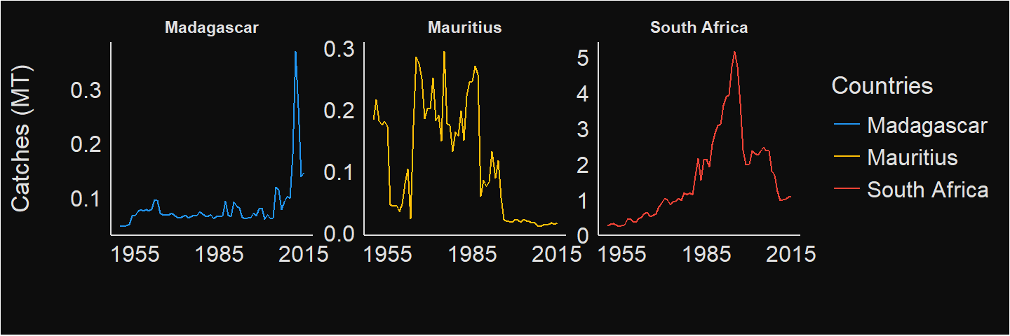
Figure 5: The three countries with the highest catches in WIO region
Species landed
The rfisheries package has a of_species_code() function that enable retrieving catches of particular species. Although the species name are given in either scientific or english name, you can only query the database using the species codes. To obtain the species code simply run a chunk below;
species = rfisheries::of_species_codes()This gives a total of 11562 species. Going through this data frame looking for a instance species of tuna is tedious. But the filter() from dplyr package (Wickham et al., 2018) only work if you can use the full variable content. But in my cases though I need to filter based on partial matches. In this case, we need a function that will evaluate regular expressions on strings and return boolean values. Whenever the statement is TRUE the row will be filtered. Fortunate, the stringr (Wickham, 2019) package has a str_detect() function that can do a partial match. However, it is important to remember that R is case sensitive. I used str_detect() below to pick tuna species name and drop other species as the code below illustrates;
tuna = species %>%
filter(str_detect(english_name %>% tolower(), pattern = "tuna"))| Scientific Name | Taxonomical Code | Species Code | English name |
|---|---|---|---|
| Gymnosarda unicolor | 1750101202 | DOT | Dogtooth tuna |
| Auxis thazard | 1750102301 | FRI | Frigate tuna |
| Auxis rochei | 1750102303 | BLT | Bullet tuna |
| Auxis thazard, A. rochei | 17501023XX018 | FRZ | Frigate and bullet tunas |
| Katsuwonus pelamis | 1750102501 | SKJ | Skipjack tuna |
| Thunnus thynnus | 1750102601 | BFT | Atlantic bluefin tuna |
| Thunnus orientalis | 1750102602 | PBF | Pacific bluefin tuna |
| Thunnus tonggol | 1750102603 | LOT | Longtail tuna |
| Thunnus atlanticus | 1750102604 | BLF | Blackfin tuna |
| Thunnus maccoyii | 1750102608 | SBF | Southern bluefin tuna |
| Thunnus albacares | 1750102610 | YFT | Yellowfin tuna |
| Thunnus obesus | 1750102612 | BET | Bigeye tuna |
| Thunnus spp | 17501026XX | TUS | True tunas nei |
| Allothunnus fallai | 1750102701 | SLT | Slender tuna |
| Thunnini | 17501XXXXX043 | TUN | Tunas nei |
| Scombroidei | 175XXXXXXX | TUX | Tuna-like fishes nei |
Once the code for species are known, we can now retrieve total annual catches for that particular species. However, notice that of_landings() only accept species code an neither the scientific name nor the english name is acceptable. The chunk below was used to extract annual catches of Yellowfin tuna shown in figure 6).
yellow.fin.tuna = rfisheries::of_landings(species = "YFT")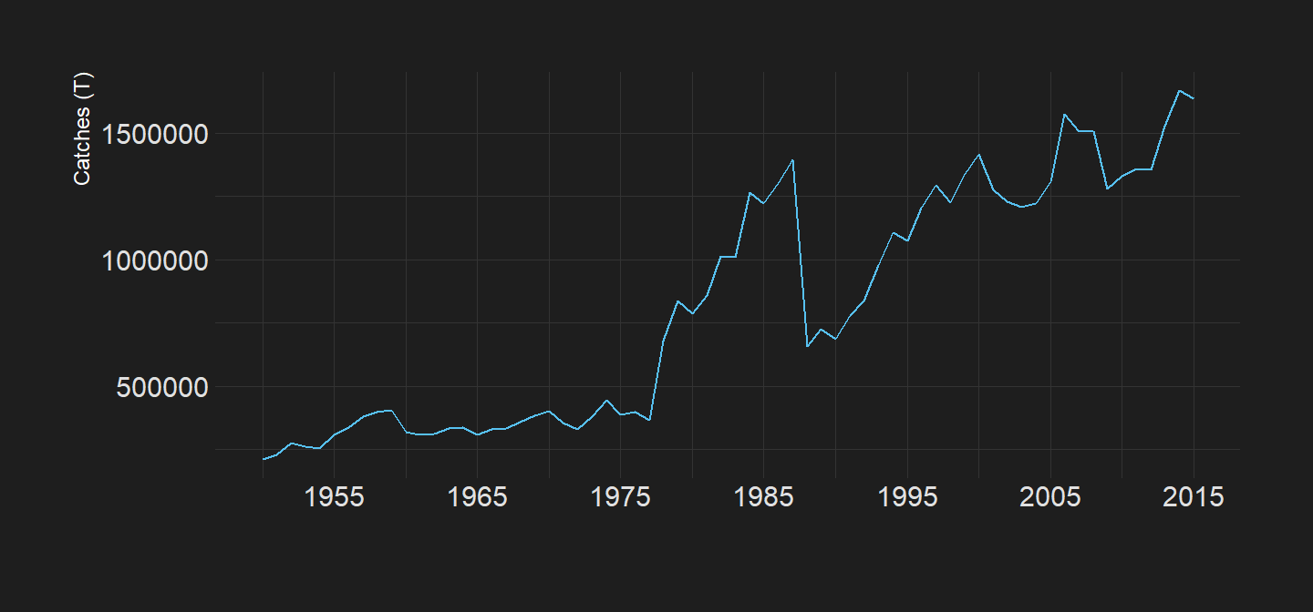
Figure 6: The globall annual catches of Yellowfin tuna
If we are interested to compare catches of multiple tuna around the world, then we must download the long–term catches data for each tuna species. With a total of 16 species that is simple and we can easily do it manually. However, that task is hard and may introduce error if you have many species to deal with. That is where looping becomes handy in programming. In this case, we use a for() loop to extract tuna and tuna like catches for all sixteen species shown in table 4. First we create a tuna_like_tuna list file as a preoccupied contain to store the data frame that has catch for each species of tuna. We also notice that Thunnus spp is vaque and the API can not recognize. Hence we need to clean the Tuna species dataset by removing missing species
## clean the dataset by removing species missing in the FAO database
tuna.clean = tuna %>%
  filter(scientific_name != "Thunnus spp")%>%
  filter(scientific_name != "Thunnini")

## create a dummy list file
tuna_like_tuna = list()

## loop through the species
for (j in 1:nrow(tuna.clean)){
  tuna_like_tuna[[j]] = rfisheries::of_landings(species = tuna.clean$a3_code[j]) %>%
    mutate(scientific_name = tuna$scientific_name[j],
           english_name = tuna.clean$english_name[j])
}

## ubind the data frame from the list
tuna_like_tuna_df = tuna_like_tuna %>% bind_rows()
Once the tuna and tuna like species catches are downloaded and in the tidy format, we can use the power of ggplot2 package to visualize catch trend of these species as shown in figure 7.
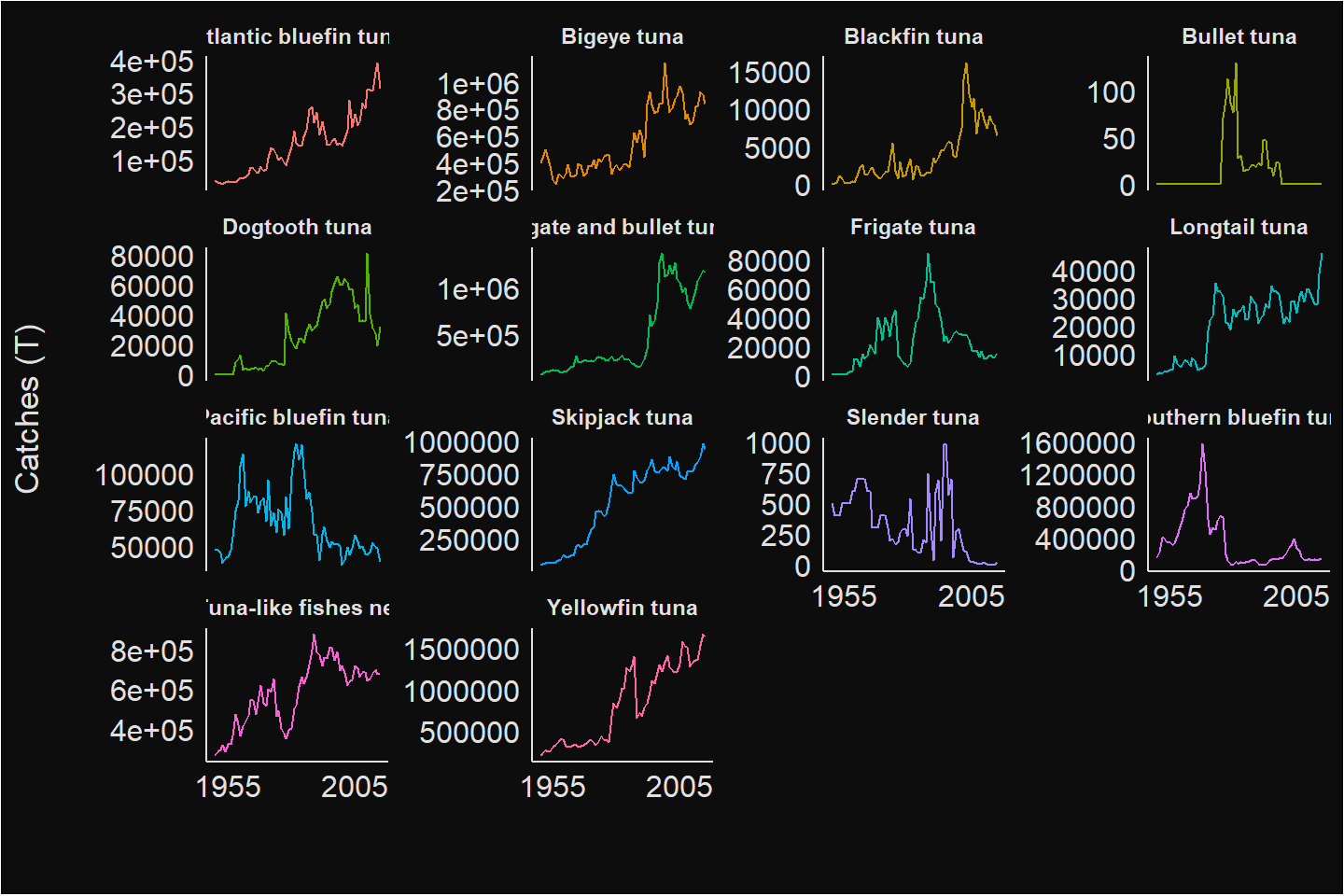
Figure 7: Trends of Global Annual total catch of Tuna and tuna like Species
Final thought
Though the rfisheries package does well to obtain the catch landing both by country and species, it only offer an opportunity to query either by species or country alone. It never allow you to query multiple variables i.e you can not fetch data like catches of certain tuna species. I hope this drawback of this package will be addressed in the future releases.
References
Müller, K., Wickham, H., 2018. Tibble: Simple data frames.
Ram, K., Boettiger, C., Dyck, A., 2016. Rfisheries: Programmatic interface to the ’openfisheries.org’ api.
R Core Team, 2019. R: A language and environment for statistical computing. R Foundation for Statistical Computing, Vienna, Austria.
Wickham, H., 2019. Stringr: Simple, consistent wrappers for common string operations.
Wickham, H., 2017. Tidyverse: Easily install and load the ’tidyverse’.
Wickham, H., François, R., Henry, L., Müller, K., 2018. Dplyr: A grammar of data manipulation.