Processing ADCP Data with R

Introduction

The Second International Indian Ocean Expedition (IIOE-2) collected various oceanographic data within the coastal water of Tanzania. Among the oceanographic data collected using Agulhas II, is the Acoustic Doppler Current Profiles (ADCP). The measurement was carried out from 4^th to 9^th November 2017. In this post, I will illustrate how to process the ADCP data with R using oce package developed by Kelley & Richards (2018). First, we need to load other packages needed for this routine using require() function (Cheng, Karambelkar, & Xie, 2018; Grolemund & Wickham, 2011; Kelley, 2015; Pebesma, 2018; Wickham, 2017).

require(oce)
require(ocedata)
require(tidyverse)
require(lubridate)
require(leaflet)
require(sf)

Ingestion of the data

Once the package needed for this routine are loaded, we can start processing the data. However, we need to import this dataset into the workspace using the read.adp() function from oce package

adp = read.adp("./AGU028002_000000.LTA")
# summary(adp)
time = adp[["time"]]

Figure 1 show the velocity of zonal (north) and meridional (east) components from the raw data as captured by the ADCP instrument. These velocities were measured along the coastal of Tanzania water from 2017-11-04 17:22:17 off Unguja Island close to Chwaka Bay and finish on 2017-11-09 02:02:23 in Mtwara.

plot(adp, which = c(1:2), 
     tformat = "%B %d, %Y:%H:%M", 
     missingColor = "grey", 
     ylim = c(25,1000),
     zlim = c(-4,6),
     useSmoothScatter = TRUE,
     ytype = "profile",
     titles = c("Northing Profiles","Northing Profiles" ),
     col = oceColorsViridis(125),
     marginsAsImage = TRUE, decimate = FALSE)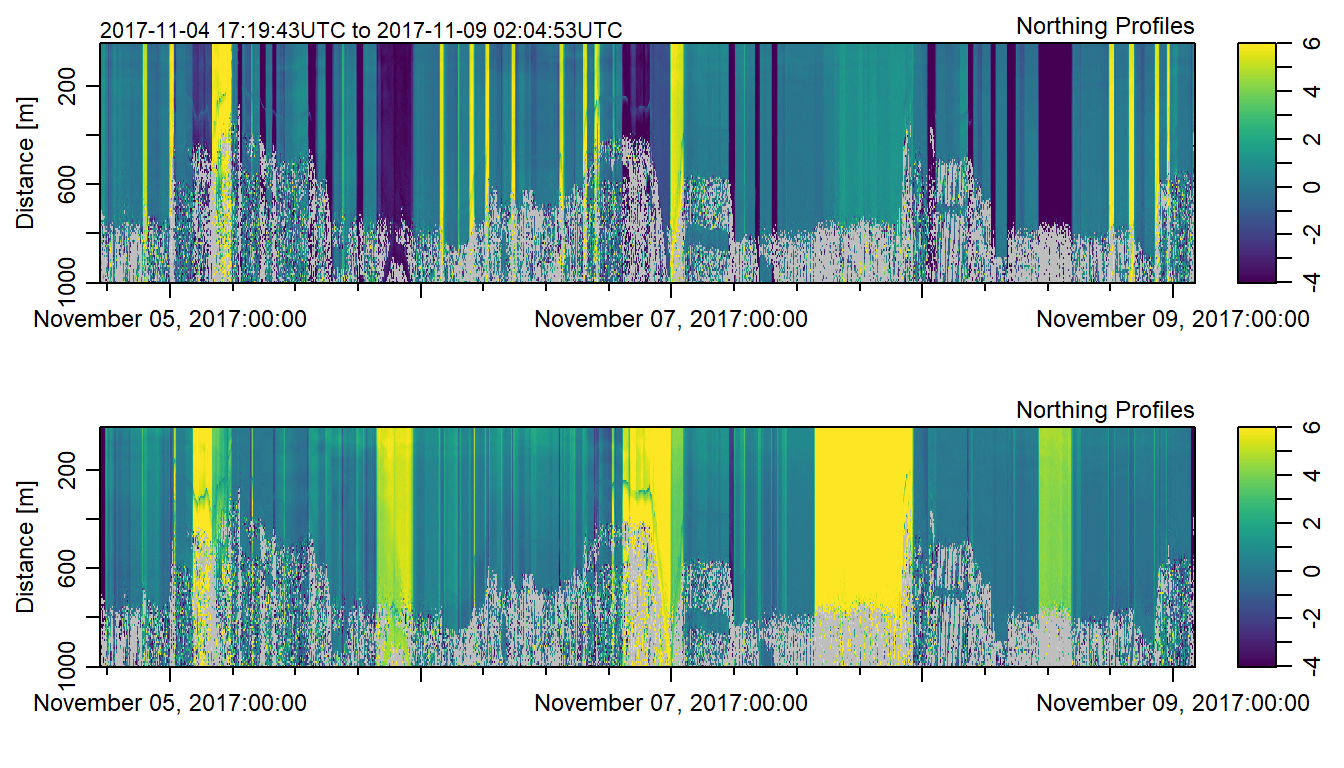

Figure 1: Meridional and Zonal components velocity before averaging the profiles

Ensemble adp objects

The grey-colored in figure 1 are bad data mostly comes from single-ping velocity. Therefore, data are averaged to reduce the measurement uncertainty to acceptable levels (Kelley & Richards, 2018). Ensemble refers as a process of averaging ping profiles from ADCP data. This approach is important because it remove the uncertainty in velocity estimates from single pings, it also reduce the size of high frequency data, which reduce processing time. I used adpEnsembleAverage() function from oce package to ensemble (average) the profiles as shown in the chunk below.

ensembled = adp%>%adpEnsembleAverage(n = 10, leftover = TRUE, na.rm = TRUE)

# summary(ensembled)

The ADCP object profiles were reduced by a factor of 10 and since they were average, the command na.rm = TRUE was parsed to ensure that profiles without values are also computed. The origin adcp file had a total of 1257 profiles, which were reduced to 126 with the adpEnsembleAverage. Figure 2 show the velocity of zonal (north) and meridional (east) components of ensembled (average ping profiles) recorded by the ADCP instrument.

plot(ensembled, which = c(1:2), 
     tformat = "%B %d, %Y:%H:%M", 
     missingColor = "grey", 
     ylim = c(25,1000),
     zlim = c(-4,6),
     useSmoothScatter = TRUE,
     ytype = "profile",
     titles = c("Northing Profiles","Northing Profiles" ),
     col = oceColorsViridis(125),
     marginsAsImage = TRUE, decimate = FALSE)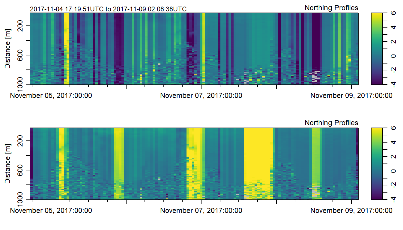

Figure 2: Meridional and Zonal components velocity after averaging the profiles

Depth cell mapping

The averaged profile (figure 2) were then aligned to the uniform depth—a process referred as depth cell mapping. Figure 3 show the cells that aligned to the standard depth. This process is important because it ensure horizontal homogeneity of cells that are at the same depth, which compensate the pitch and roll of the instrument during ship cruising. This only works for adcp data that are in beam coordinates.

ensembled.bin = binmapAdp(ensembled)

## plot the ensembled
plot(ensembled.bin, which = c(1:2), 
     tformat = "%B %d, %Y:%H:%M", 
     missingColor = "grey", 
     ylim = c(25,1000),
     zlim = c(-4,6),
     useSmoothScatter = TRUE,
     ytype = "profile",
     titles = c("Northing Profiles","Northing Profiles" ),
     col = oceColorsViridis(125),
     marginsAsImage = TRUE, decimate = FALSE)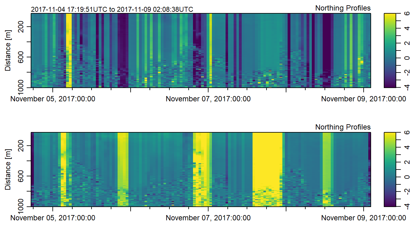

Figure 3: Meridional and Zonal components velocity after averaging the profiles and align to standard depth

Extract the variables

Figure 4 show the sampled location of ADCP profile pings.

Subset ADCP

Since I am interested on the current between Lindi and Mafia Island (Figure 5), I ought to chop the pings that fall within the area. Unfortunately the function subset(), which I used, only capable of chopping adcp data using either time or distance. Based on figure 4, only the pings profiles within the areas were selected by visual inspection of the points on the map and then use the date file to filter those pings with subset() function. Once the pings were selected, then distance, longitude, latitude, v, u were extracted. Using the u and v component, the velocity was computed with the equation (1)

\[ \begin{equation} Velocity (ms^{-1})\:=\: \sqrt{(U^2+V^2)} \tag{1} \end{equation} \]

## creae a date limit
date = c("2017-11-07 13:14:52", "2017-11-07 23:14:51")%>%as_datetime()

## subset to the area based on date limit,
kilwa.adcp = ensembled.bin%>%subset(time >= date[1] & time <= date[2])%>%subset(distance < 700)

## extract variables from the subset
time = kilwa.adcp[["time"]]
distance = kilwa.adcp[["distance"]]
lon = kilwa.adcp[["firstLongitude"]]
lat = kilwa.adcp[["firstLatitude"]]
v = kilwa.adcp[["v"]][,,1]
u = kilwa.adcp[["v"]][,,2]

vel = sqrt(v^2 + u^2)

## make sf feature
kilwa.sf = data.frame(lon,lat,time)%>%st_as_sf(coords = c("lon", "lat"))%>%st_set_crs(4326)

## plot the location of ADCP
leaflet(data = kilwa.sf)%>%
  addTiles()%>%
  addMarkers(popup = ~time)

Figure 6 show ocean current between Lindi and Mafia Island (figure 5) decrease with depth. The current at the surface is strong and decrease gradually with increase in depth. We also notice the current becomes more strong from Lindi toward Mafia, this can be contributed by the East African Coastal Current (McClanahan, 1988).

## plot the velocity profiles as section
imagep(lat,distance, vel, filledContour = TRUE, 
       ylim = c(700, 30), zlim = c(6,7.0), zclip = TRUE, 
       col = oceColors9A(120), xlim = c(-9.5, -8.3), 
       xlab = "Latitude", ylab = "Depth (meters)", 
       zlab = "Current Velocity [m/s]", zlabPosition = "side")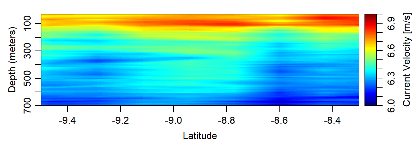

Figure 6: Current Profile

Spurious measurements

Looking on individual profiles, We noticed that the current velocity deviate from what has been reported previously. Setting cut point of equal or less than 1 ms^-1, we found that only the first profile had TRUE value— met the criterion, other profile had FALSE implying the current of these profiles are above 1 ms^-1 (Figure 7).

# create profiles
kilwa.profile = vel %>% 
   # transpose
  t() %>% 
  # convert to data frame
  as.data.frame() %>%
  # make it tibble
  as.tibble()

## change variable names
colnames(kilwa.profile) =  paste("profile", 1:12, sep = "")

## bind the disance to the profile
kilwa.profile = data.frame(distance, kilwa.profile)

## make it long form from wide form
kilwa.profile.long = kilwa.profile %>%
  gather(key = "profile", value = "velocity", 2:13)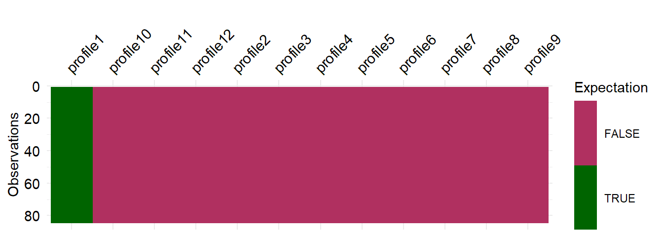

Figure 7: Profile with velocity above 1 m/s

Similar to Figure 7, which showed the profile one as true value and assigned other profile as false because of current value above the criterion of 1 ms^-1, figure 8 show the actual current value of each profile along the transect from Lindi to Mafia. All profiles except profile measured at location with latitude -8.0252 and longitude 40.0961 (figure 9) have current speed above 1 ms^-1. This is a relative current velocity values, which is significantly higher than the actual speed in the area. Therefore, we ought to convert relative speed to absolute velocity to obtain the actual current velocity.

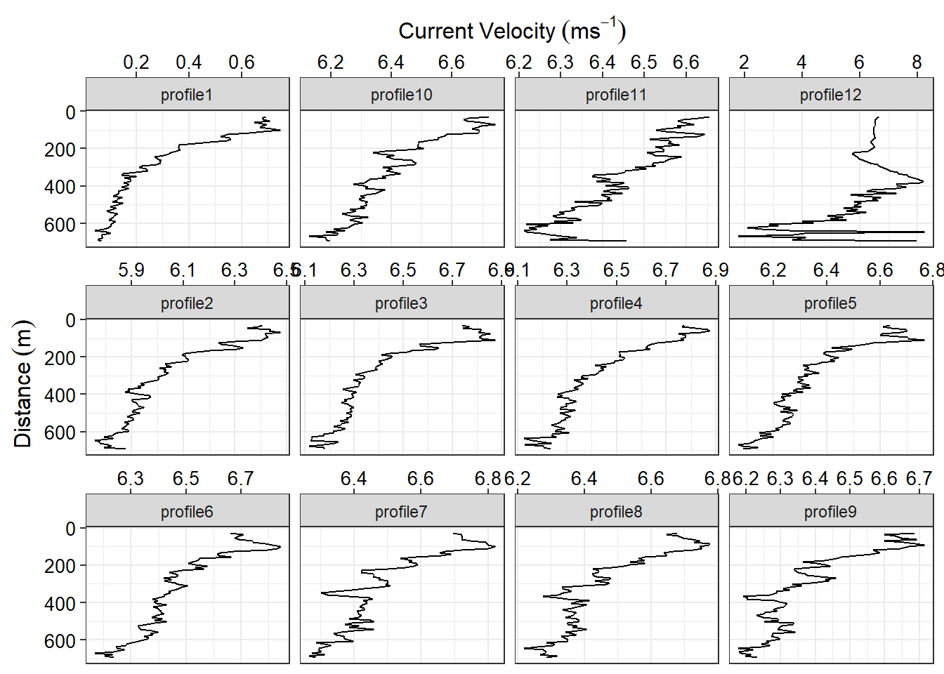
Figure 8: Current profiles at each ping

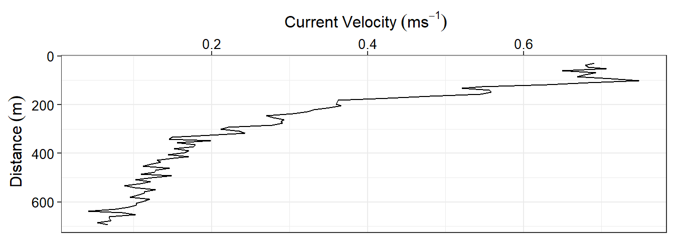
Figure 9: profile at station 1

Compute Absolute velocity

The ADCP measure a relative velocity to the earth, to obtain an absolute velocity, we need to substract the relative velocity with the ship velocity using the mathematical equation (2)

\[ \begin{equation} \beta \: = \gamma\: - \epsilon \: \tag{2} \end{equation} \] where; \(\beta\) = absolute velocity; \(\gamma\) = relative velocity; \(\epsilon\) = ship velocity

The mathematical equation (2) was used to compute the absolute velocity in R involves two-steps as illustrated in the chunk below. First the ship velocity was determined at each profile ping. Second, the relative velocity was substracted with this ship velocity to obtain absolute velocity.

##  calculate ship velocity 
ship.vel = kilwa.adcp[["avgSpeed"]]
## obtain absolute velocity
vel.abs = abs(vel-ship.vel)

After ship correction, the profiles of absolute current velocity ranged from 1.493310^{-4} ms^-1 to 4.647 ms^-1 with the median of 0.1234 ms^-1 (figure 10). Stitching the profile together and create a section, we noticed a decline of current speed with increase in depth where the surface water has a relatively higher current speed than the deep water (figure 11). It also clear the surface current velocity increase from Lindi to around latitude 9 ^oS has relatively lower surface current and increases from 8 ^oS toward Mafia (figure 11), which might be caused by East African Coastal Current.

# create profiles
abs.vel.profile = vel.abs %>% 
   # transpose
  t() %>% 
  # convert to data frame
  as.data.frame() %>%
  # make it tibble
  as.tibble()

## change variable names
colnames(abs.vel.profile) =  paste("profile", 1:12, sep = "")

## bind the disance to the profile
abs.vel.profile = data.frame(distance, abs.vel.profile)

## make it long form from wide form
abs.vel.profile.long = abs.vel.profile %>%
  gather(key = "profile", value = "velocity", 2:13)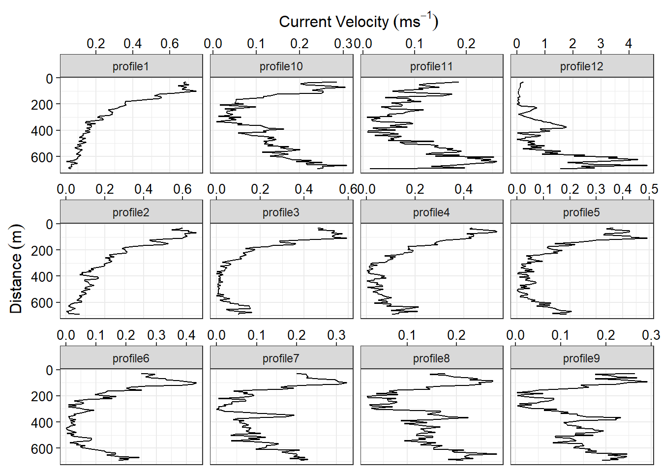

Figure 10: Current profiles at each ping

## plot the velocity profiles as section

imagep(lat,distance, vel.abs, filledContour = TRUE, 
       ylim = c(30, 700), zlim = c(0,.6), zclip = TRUE, flipy = TRUE,
       col = oceColors9A(120), xlim = c(-9.5, -8.3), 
       xlab = "Latitude", ylab = "Depth (meters)", 
       zlab = "Current Velocity [m/s]", zlabPosition = "side",
       at = seq(0.04, 0.58, length.out = 6)%>%round(digits = 2), 
       drawPalette = TRUE, drawTriangles = TRUE)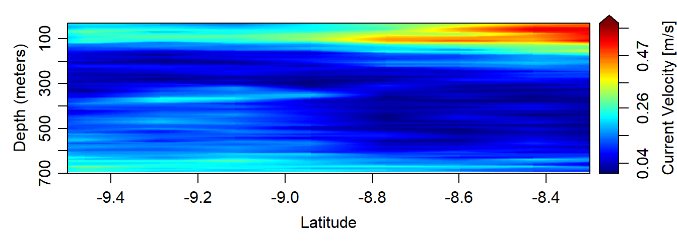

Figure 11: ADCP profile current Velocity between Lindi and Mtwara after correction of the ship speed

Conclusion

Unlike current meters, ADCP collect current velocity along the vertical and horizontal dimension, hence provide detailed water column circulation. Given the ongoing current measurement with the IIOE-2, we see oce package in R offers and alternative option of CODAS to ingest, process, manipulate and visualize ADCP data under one roof.