Introduction
in the previous post, we looked at CTD processing and visualization of profile and section with oce package. We saw the necessary tools needed to import, transform and even plotting oceanographic standard graphics. This post introduce to an ecosystem of packages called tidyverse. The three packages in tidyverse that people use in everyday data analyses include the grammer for graphic ggplot develop by Wickham (2016) for data visualization. The second package is tidyr (Wickham & Henry, 2018) for tidying data in consistent ways for analysis and the third package is dplyr (Wickham, François, Henry, & Müller, 2018) for data wringling. we load these packages in R first if not installed, please install it first from CRAN.
require(tidyverse)
require(oce)
require(leaflet)
require(sf)
Now that we have loaded the packages, its time to import the CTD data. we load the ctd files with oce::read.ctd() function. CTD files don’t have the longitude and latitude information of the casts, these geographical information were collected separately using a GPS device. We also load the locations data with readr::read_csv() function
ctd = read.ctd("./ctd_rufiji/SBE19plus_01906740_2018_02_13_0885.cnv")
cast.locations = read_csv("./ctd_rufiji/Rufiji_cast.csv")
Table 1 give a summary of the geographical information of each CTD cast. It contains five variable that inform whether the cast was done during the morning or evening and whether is during the low or high tide; the assigned station code together with longitude and latitude.
cast.locations%>%select(Time, Tide, Name, Lon, Lat)%>%sample_n(10)%>%
  knitr::kable("html",caption = "Location information of CTD casts done during the low and high Tide in Rufiji River",
               digits = 4, align = "c")%>%
  kableExtra::kable_styling(bootstrap_options = c("striped", "hover", "condensed", "responsive"))%>%
  kableExtra::column_spec(1:5,width = "8cm", color = 1)%>%
  kableExtra::add_header_above(c("Station Information" = 3,
"Location information" = 2))| Time | Tide | Name | Lon | Lat |
|---|---|---|---|---|
| Evening | High | St17 | 39.2692 | -7.8073 |
| Morning | Low | St41 | 39.2868 | -7.7948 |
| Evening | High | St3 | 39.3123 | -7.7364 |
| Morning | Low | St53 | 39.3161 | -7.7353 |
| Evening | High | s10 | 39.2925 | -7.7738 |
| Morning | High | St27 | 39.2460 | -7.8578 |
| Morning | Low | St45 | 39.2925 | -7.7738 |
| Morning | Low | St38 | 39.2692 | -7.8073 |
| Morning | Low | St34 | 39.2566 | -7.8140 |
| Evening | High | st11 | 39.2938 | -7.7775 |
We add the location information into the oce object. Before we add this information we need to remove the upcast profile with ctdTrim() and also align the downcast profile at 10 cm interval from the surface the maximum depth of the cast with ctdDecimate(). Figure 1 give us a glimpse of temperature and salinity profile measured at station 1. A much detail of the station CTD information is provided in the summary below.
ctd = ctd%>%ctdTrim(method = "downcast")%>%ctdDecimate(p = 0.1)
ctd[["latitude"]] = cast.locations$Lat[1]
ctd[["longitude"]] = cast.locations$Lon[1]
par(mfrow = c(1,2))
ctd%>%plot(which = 1)
ctd%>%plot(which = "map")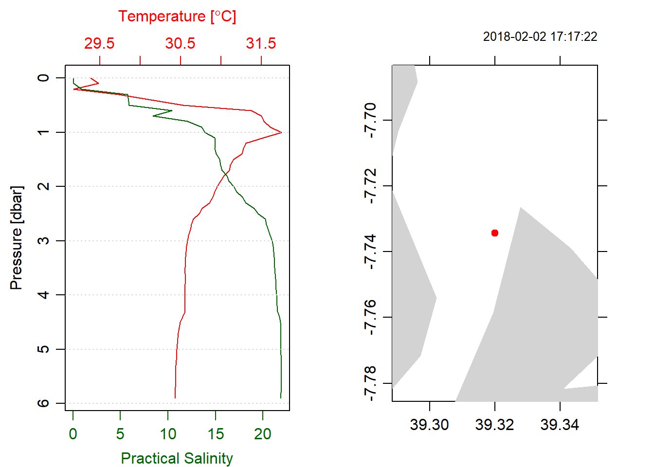
Figure 1: Profiles of temperature and salinity at station 1
summary(ctd)## CTD Summary
## -----------
##
## * Instrument: SBE
## * Temp. serial no.: 6740
## * Cond. serial no.: 6740
## * Original file: c:\users\all user\desktop\ctd tafiri 2018\sbe19plus_01906740_2018_02_13_0885.hex
## * Start time: 2018-02-02 17:17:22
## * Sample interval: 0.25 s
## * Location: 7.7344S 39.32E
## * Data
##
## Min. Mean Max. Dim. OriginalName
## pressure [dbar, Strain Gauge] 0 2.95 5.9 60 prdM
## temperature [°C, ITS-90] 29.178 30.671 31.742 60 tv290C
## conductivity [S/m] 0.011834 3.1912 3.8697 60 c0S/m
## salinity [PSS-78] 0.056455 17.781 21.925 60 sal00
## oxygen [ml/l, SBE43] 2.7495 3.422 7.9216 60 sbeox0ML/L
## fluorescence [mg/m³, WET Labs] -0.0509 1.959 3.3368 60 flECO-AFL
## bottlesFired 0 0 0 60 nbf
## time2 [day, elapsed] 33.72 33.721 33.722 60 timeJ
## density [kg/m³] 995.85 1008.7 1011.8 60 density00
## depth [m] 0.042 2.977 5.847 60 depSM
## descentRate [m/s] -0.047 0.11817 0.257 60 dz/dtM
## scan 11.9 304.66 456.89 60 -
##
## * Processing Log
## - 2018-10-05 13:40:55 UTC: `create 'ctd' object`
## - 2018-10-05 13:40:56 UTC: `read.ctd.sbe(file = file, columns = columns, station = station, missingValue = missingValue, monitor = monitor, debug = debug, processingLog = processingLog)`
## - 2018-10-05 13:40:56 UTC: `ctdTrim(x = ., method = "downcast")`
## - 2018-10-05 13:40:56 UTC: `ctdDecimate(x = ., p = 0.1)`
## - 2018-10-05 13:40:56 UTC: `Removed flags from decimated ctd object`
## - 2018-10-05 13:40:56 UTC: `Removed flag field from decimated ctd object`Oce object tibble
Thoroughout the post we have been working with oce object, which implement the object-oriented programming (OOP). Unfortunate tidyverse cant work with oce object directly but rather work with data frame, and prefer a tabular data converted to tibble. Wickham & Grolemund (2016) defined a tibble as a modern data frame. of the three slots in oce object—metadata, data and processinglog, the profile information are contained in the data slot. Therefore, this is the slot that was transformedto tibble with as_data_frame() function. Note the use of pipe %>%, the handiest operator in the tidyverse.
ctd.tb = ctd@data%>%
  as_data_frame()
Wrangle the data
The tibble obtained through transformation of oce object contains only numerical data. Other ancillary information can be added into the tibble from the metadata slot. I added a column of time for which the CTD measurement was done using dplyr’s function mutate() . Because the CTD records time and date as one entity, I separate the date and time as individual variables with the tidyr’s function `separate()’. Then only variable of interest were retained (Table 2), the rest were removed form the dataset.
ctd.tb = ctd.tb %>%
  mutate(datetime = ctd@metadata$time,
         lon = ctd@metadata$longitude,
         lat = ctd@metadata$latitude) %>%
  separate(datetime, c("date", "time"), sep = " ")%>%
select(date, time, lon,lat,pressure,temperature, salinity, oxygen, fluorescence)| Date | Time | Longitude | latitude | Pressure | Temperature | Salinity | Oxygen |
|---|---|---|---|---|---|---|---|
| 2018-02-13 | 13:57:46 | 39.32 | -7.73 | 0.0 | 29.39 | 0.06 | 3.74 |
| 2018-02-13 | 13:57:46 | 39.32 | -7.73 | 0.3 | 29.74 | 5.72 | 4.28 |
| 2018-02-13 | 13:57:46 | 39.32 | -7.73 | 0.6 | 31.37 | 10.39 | 2.84 |
| 2018-02-13 | 13:57:46 | 39.32 | -7.73 | 0.9 | 31.61 | 13.53 | 3.23 |
| 2018-02-13 | 13:57:46 | 39.32 | -7.73 | 1.2 | 31.30 | 14.95 | 2.78 |
| 2018-02-13 | 13:57:46 | 39.32 | -7.73 | 1.5 | 31.16 | 15.41 | 2.89 |
| 2018-02-13 | 13:57:46 | 39.32 | -7.73 | 1.8 | 31.03 | 16.18 | 3.81 |
| 2018-02-13 | 13:57:46 | 39.32 | -7.73 | 2.1 | 30.92 | 17.23 | 3.40 |
| 2018-02-13 | 13:57:46 | 39.32 | -7.73 | 2.4 | 30.76 | 19.08 | 2.84 |
| 2018-02-13 | 13:57:46 | 39.32 | -7.73 | 2.7 | 30.63 | 20.38 | 3.24 |
| 2018-02-13 | 13:57:46 | 39.32 | -7.73 | 3.0 | 30.58 | 20.96 | 3.51 |
| 2018-02-13 | 13:57:46 | 39.32 | -7.73 | 3.3 | 30.56 | 21.16 | 3.57 |
| 2018-02-13 | 13:57:46 | 39.32 | -7.73 | 3.6 | 30.56 | 21.28 | 3.67 |
| 2018-02-13 | 13:57:46 | 39.32 | -7.73 | 3.9 | 30.56 | 21.40 | 3.41 |
| 2018-02-13 | 13:57:46 | 39.32 | -7.73 | 4.2 | 30.55 | 21.49 | 3.30 |
| 2018-02-13 | 13:57:46 | 39.32 | -7.73 | 4.5 | 30.50 | 21.82 | 3.41 |
| 2018-02-13 | 13:57:46 | 39.32 | -7.73 | 4.8 | 30.46 | 21.89 | 3.44 |
| 2018-02-13 | 13:57:46 | 39.32 | -7.73 | 5.1 | 30.45 | 21.91 | 3.41 |
| 2018-02-13 | 13:57:46 | 39.32 | -7.73 | 5.4 | 30.44 | 21.92 | 3.44 |
| 2018-02-13 | 13:57:46 | 39.32 | -7.73 | 5.7 | 30.44 | 21.92 | 3.44 |
Plotting the Profiles
The ggplot2 package which is part of the tidyverse use a grammer of graphic to make elegant graphic that meet oceanographic standard. For instance, figure 2 present profiles of temperature, salinity and oxygen plotted with ggplot2. Wilke (2018) developed a cowplot package that I used it’s function plot_grid() to combine the three profile plots.
temp = ggplot(data = ctd.tb%>%na.omit(),
       aes(x = temperature, y = pressure))+
  geom_path( col = "red")+
  scale_y_reverse(breaks = seq(0,7,1.5))+
  scale_x_continuous(breaks = seq(28.5,33,1.25), position = "top")+
  theme_bw()+
  theme(axis.text = element_text(size = 12, colour = 1),
        axis.title = element_text(size = 14, colour = 1))+
  labs(x = expression(~Temperature~(degree~C)), y = "Pressure[dbar]")


salinity = ggplot(data = ctd.tb%>%na.omit(),
       aes(x = salinity, y = pressure))+
  geom_path( col = "darkgreen")+
  scale_y_reverse(breaks = seq(0,7,1.5))+
  scale_x_continuous(breaks = seq(4,25,8), position = "top")+
  theme_bw()+
  theme(axis.text = element_text(size = 12, colour = 1),
        axis.title = element_text(size = 14, colour = 1))+
  labs(x = expression(~Practical~salinity),
       y = expression(~Pressure~(dbar)))

oxygen = ggplot(data = ctd.tb%>%na.omit(),
       aes(x = oxygen, y = pressure))+
  geom_path( col = "blue")+
  scale_y_reverse(breaks = seq(0,7,1.5))+
  scale_x_continuous(breaks = seq(0,8,1.5), position = "top")+
  theme_bw()+
  theme(axis.text = element_text(size = 12, colour = 1),
        axis.title = element_text(size = 14, colour = 1))+
  labs(x = expression(~DO~(mgL^{-3})),
       y = expression(~Pressure~(dbar)))

cowplot::plot_grid(temp,salinity, oxygen, nrow = 1)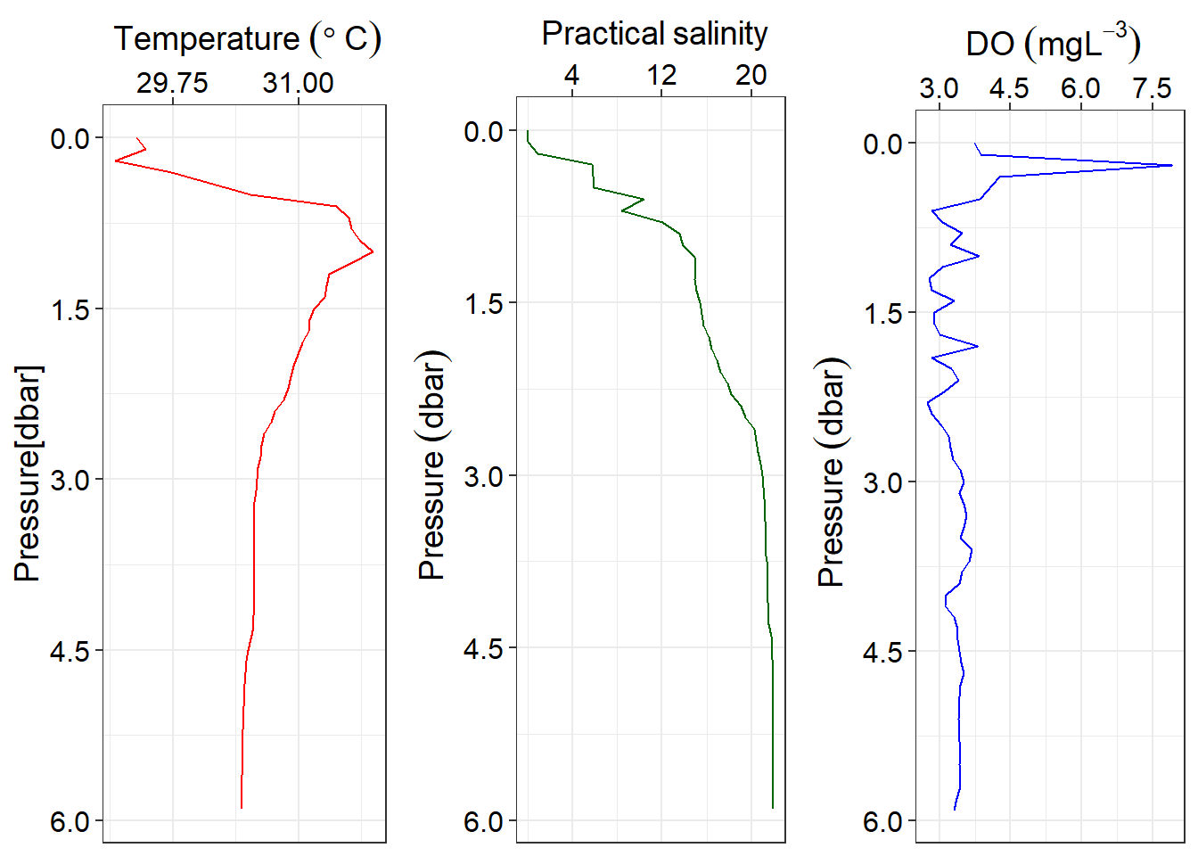
Figure 2: Profiles of temperature, salinity and oxygen plotted with ggplot2 package
Conclusion
We have seen in this post on how to process CTD data with oce and tidyverse package of a station in the mouth of Rufiji River shown in static map in Figure 3 and its interactive one in figure 4. The post illustrate that there many ways to plot the profile, so what matters depend on the package that makes you comfort while coding. A si
# tz = st_read("./africa.shp")

ggplot()+
  geom_sf(data = tz, fill = "ivory", col = 1)+
  coord_sf(xlim = c(39.28, 39.4) , ylim = c(-7.77,-7.70))+
  geom_point(data = cast.locations%>%slice(1), aes(x = Lon, y = Lat), size = 6 )+
  geom_label(data = cast.locations%>%slice(1),
             aes(x = Lon-0.006, y = Lat+0.006, label = Name))+
  theme_bw()+
  theme(axis.text = element_text(size = 12, colour = 1),
        panel.background = element_rect(fill = "lightblue"))+
  scale_x_continuous(breaks = c(39.3,39.39))+
  scale_y_continuous(breaks = c(-7.76,-7.71))+
  geom_text(aes(x = 39.35, y = -7.72, label = "Rufiji River Estuary"), col = "white", size = 5)+
  labs(x = "", y = "")+
  ggsn::scalebar(location = "bottomright", x.min = 39.3, x.max = 39.4, y.min = -7.765, y.max = -7.71, dist = 1.5, dd2km = TRUE, model = "WGS84", st.dist = 0.04, st.size = 4, height = 0.04)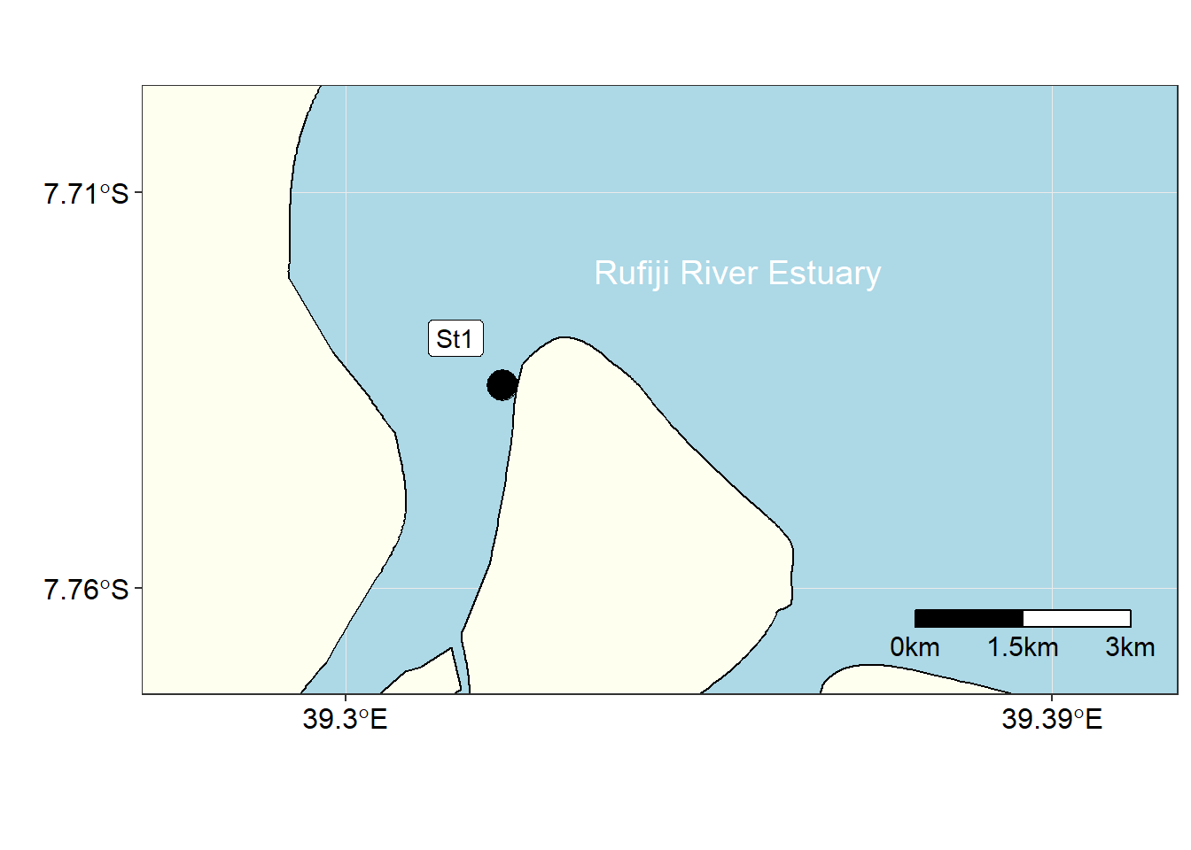
Figure 3: Location of Station 1
#ggsn::north2(x = 0.65,y = .95, scale = .1, symbol = 8)leaflet(data = cast.locations%>%slice(1))%>%
setView(lng = 39.3, lat = -7.73, zoom = 10)%>%
addTiles() %>%
# addProviderTiles("Stamen.Watercolor") %>%
addMarkers(lng = ~Lon, lat = ~Lat, popup = ~Name)Figure 4: Location of Station 1
References
Wickham, H. (2016). Ggplot2: Elegant graphics for data analysis. Springer-Verlag New York. Retrieved from http://ggplot2.org
Wickham, H., & Grolemund, G. (2016). R for data science: Import, tidy, transform, visualize, and model data. “ O’Reilly Media, Inc.”
Wickham, H., & Henry, L. (2018). Tidyr: Easily tidy data with ’spread()’ and ’gather()’ functions. Retrieved from https://CRAN.R-project.org/package=tidyr
Wickham, H., François, R., Henry, L., & Müller, K. (2018). Dplyr: A grammar of data manipulation. Retrieved from https://CRAN.R-project.org/package=dplyr
Wilke, C. O. (2018). Cowplot: Streamlined plot theme and plot annotations for ’ggplot2’. Retrieved from https://CRAN.R-project.org/package=cowplot