Processing CTD data with OCE package in R

Importing CTD Data

SBE comes with SBE Data Processing Graphic User Interface to help converting the data from binary to engineering unit. I use this software to convert .hex raw data from CTD and store them in .cnv file format. Once the file was ready, I imported it from local folder into R workspace with read.ctd() function. according to Kelley & Richards (2018)

read.ctd() is a base function that read different format of CTD data including read.ctd.odf for the ODF data used in Fisheries and Oceans (Canada), read.ctd.woce for data in World Ocean Circulation Experiment format, read.ctd.woce.other for a variant of WOCE data, read.ctd.itp for ice-tethered-profiler data, or read.ctd.sbe for Seabird data.

#read profile of station1
stn1 = read.ctd("./ctd_rufiji/SBE19plus_01906740_2018_02_13_0885.cnv")

oce organize the CTD object into three slots—metadata, data and processing log.

• metadata: a list with information about the data like units, quality, sampling location, sampling time, …etc
• data: a list of raw profile data like pressure, temperature, salinity.
• processinglog: a document track all the processing information

str(stn1,2)

## Formal class 'ctd' [package "oce"] with 3 slots
##   ..@ metadata     :List of 27
##   ..@ data         :List of 13
##   ..@ processingLog:List of 2

Depending on configuration, the content in CTD file differs . But the data slots often remain fairly constant with the content. For instance, here we see the data slots with thirteen variables and six hundreds and sixteen observations for profiles in station_1.

stn1@data%>%as.data.frame()%>%dplyr::glimpse()

Observations: 616
Variables: 13
$ pressure     <dbl> 0.074, 0.074, 0.063, 0.074, 0.074, 0.074, 0.064, ...
$ temperature  <dbl> 29.6868, 29.6889, 29.6911, 29.6922, 29.6925, 29.6...
$ conductivity <dbl> 0.008290, 0.008492, 0.008459, 0.008810, 0.008703,...
$ salinity     <dbl> 0.0419, 0.0427, 0.0426, 0.0440, 0.0435, 0.0444, 0...
$ oxygen       <dbl> 3.6746, 3.5385, 3.9256, 3.5252, 3.4002, 3.3936, 3...
$ fluorescence <dbl> 0.5136, 0.5091, 0.5068, 0.5144, -0.0227, -0.0166,...
$ bottlesFired <int> 0, 0, 0, 0, 0, 0, 0, 0, 0, 0, 0, 0, 0, 0, 0, 0, 0...
$ time         <dbl> 0.00, 0.25, 0.50, 0.75, 1.00, 1.25, 1.50, 1.75, 2...
$ time2        <dbl> 33.72039, 33.72040, 33.72040, 33.72040, 33.72040,...
$ density      <dbl> 995.7750, 995.7749, 995.7741, 995.7749, 995.7745,...
$ depth        <dbl> 0.074, 0.074, 0.063, 0.074, 0.074, 0.074, 0.063, ...
$ descentRate  <dbl> -2.632e-17, 0.000e+00, -3.000e-03, -2.000e-03, -1...
$ flag         <dbl> 0, 0, 0, 0, 0, 0, 0, 0, 0, 0, 0, 0, 0, 0, 0, 0, 0...

Visualising Profiles

Looking on those number seems boring, let us take a quick gander at those number by making profile plots. Figure 1 shows the profiles of CTD measurements at station one. At top left and right we have some waer column profiles of temperature, salinity and density. At the bottom left is the temperature-salinity plot with contours of density.

#plot
stn1%>%plot()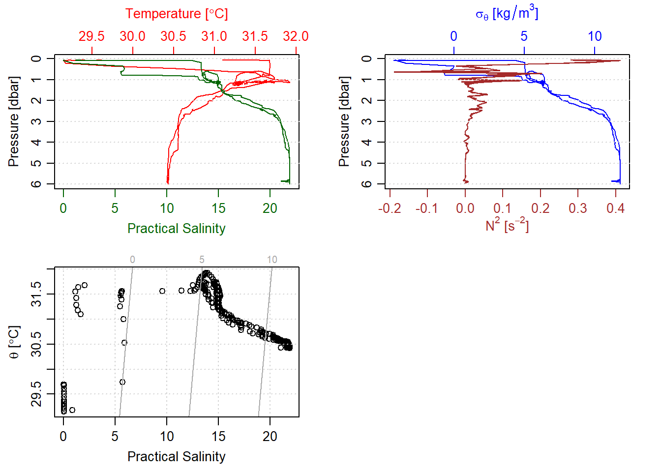

Figure 1: Unprocessed CTD measurement

Unfortunately CTD data for station one does not have a location data. This is because GPS information was not integrated into the SBE equipment. However, the location information were collected separately using a handheld GPS unit. I added this information manually for the station one.

cast.locations = read.csv("./ctd_rufiji/Rufiji_cast.csv")

stn1[["longitude"]] = cast.locations$Lon[1]
stn1[["latitude"]] = cast.locations$Lat[1]

Plotting the CTD data that contain location information, often times plot a map showing the location of the CTD cast. Figure 2 is similar to to 1, except the bottom right has been added in this plot, which show where and when the cast was done.

stn1%>%plot()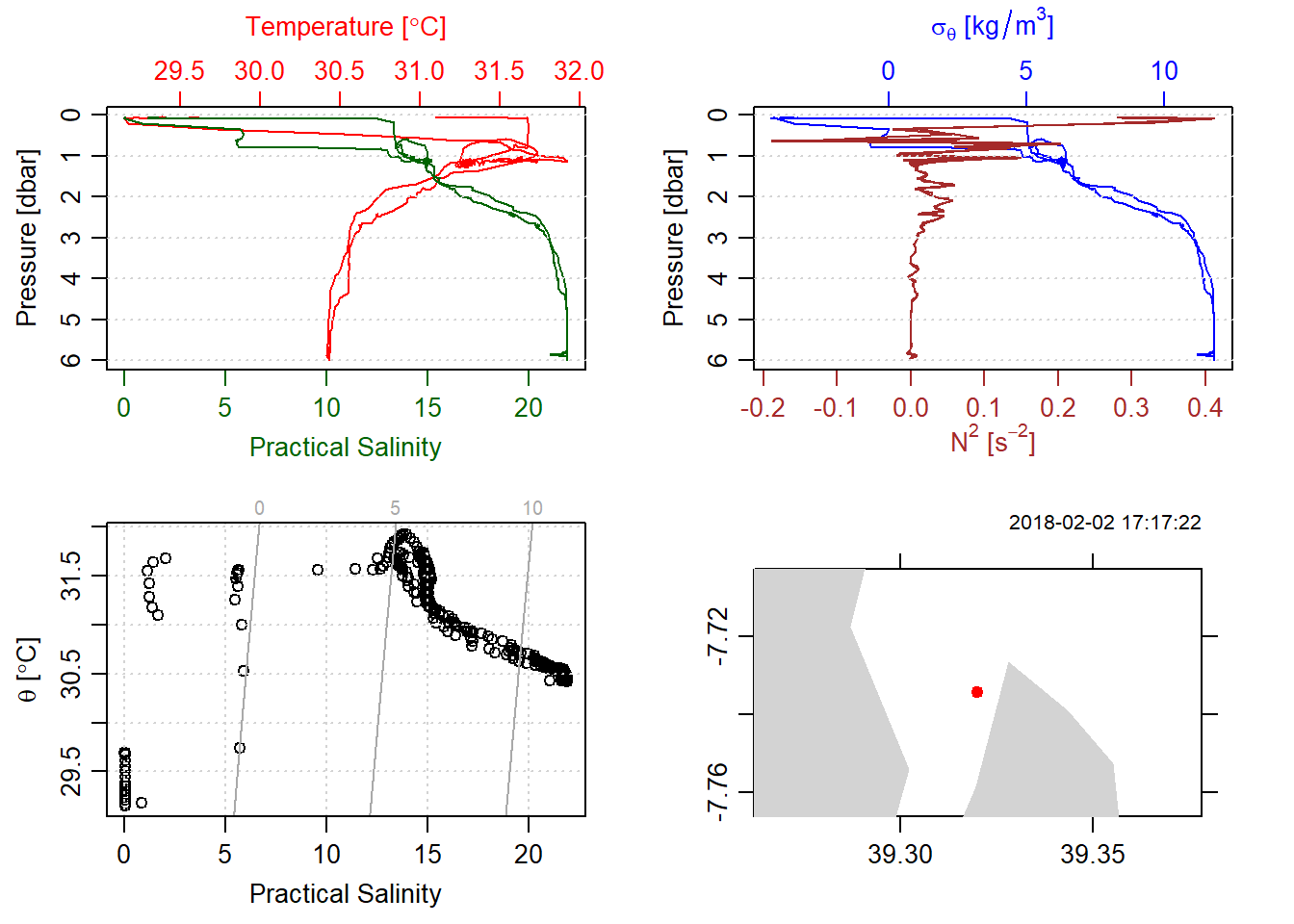

Figure 2: CTD data with location information

When we glimpse the salinity and temperature profile (Figure 3), we can see that there are profile measurements from downcast and upcast. Often in CTD profiling, the goal is to retain the downcast and drop all measurement from the upcast. The other thing you notice for figure 3 is the downcast and upcast profile of temperature and salinity are not smooth and sharp. This is because the rate of towing CTD instrument differs with because it was done manually.

par(mfrow = c(1,2))
stn1%>%plot(which = "salinity")
stn1%>%plot(which = "temperature")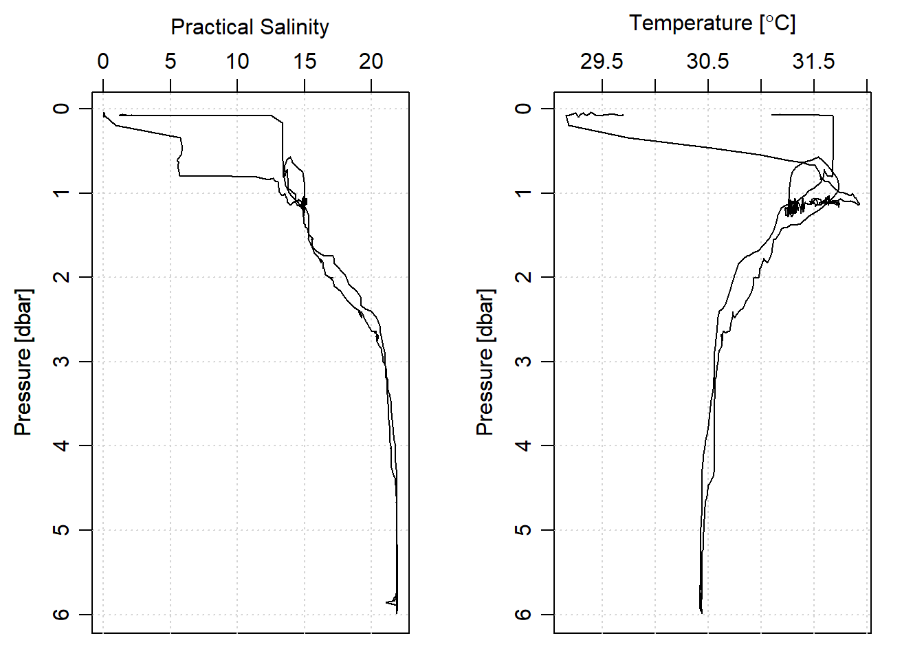

Figure 3: Salinity and temperature profiles showing downcast and upcast measurments

I removed the upcast CTD profiling with the ctdTrim() function and retained the downcast profiles. Once the upcast was dropped, I removed the artifacts introduced by towing rate. This was done by aligning the CTD measurements into the standard depth of 20 cm from the surface to the maximum depth of the cast with ctdDecimate() function. This produced elegant looking salinity and temperature profiles (Figure 4)

stn1.downcast = stn1%>%
  ctdTrim(method = "downcast")%>%
  ctdDecimate(p = 0.2)

par(mfrow = c(1,2))
stn1.downcast%>%plot(which = c("salinity"))
stn1.downcast%>%plot(which = c("temperature"))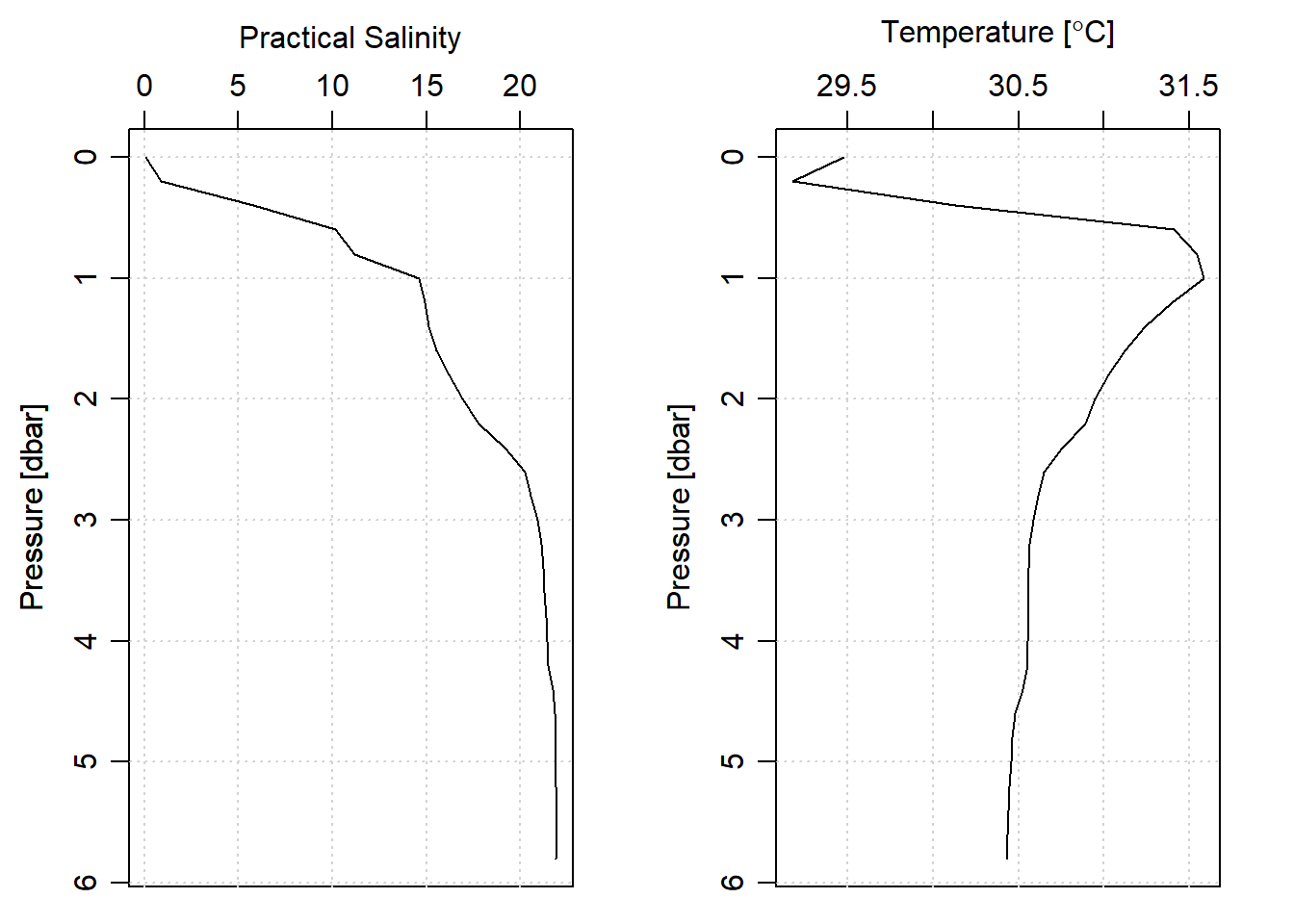

Figure 4: Profile o Salinity and temperature from downcast measurments and aligned to standard depth

plotting hydrographic section

The procedures above was just for one station, but hydrographic section involves multiple profiles. Therefore, we will loop through all the stations with a for() loop to read the `.cnv’ file, add the latitude and longitude for each cast

# create a list of cnv files
files = dir("./ctd_rufiji/", full.names = TRUE, pattern = ".cnv")

Before looping, I preallocated a list files that will store each processed CTD cast in a list. The chunk below show the processed of looping CTD data. In a nutshell, it first read the file, then remove the upcast profile and align the profile measurement to a standard pressure of 20 centimeters. Then add the longitude and latitude information for each cast.

# loop through the files
ctd = list()

for (i in 1:18){

ctd[[i]] = read.ctd(files[i])%>%
  ctdTrim(method = "downcast")%>%
  ctdDecimate(p = 0.2)

ctd[[i]][["longitude"]] = cast.locations$Lon[i]
ctd[[i]][["latitude"]] = cast.locations$Lat[i]
ctd[[i]][["stations"]] = cast.locations$Name[i]


}

Once we have a list of all the files, we can create a section along the river that only use the center positions of each cast. We notice that the CTD measurements was done at the middle of the within the channel with depth ranged from 3 to 9 meters.

section = list(ctd[[2]],ctd[[5]],ctd[[8]],
                         ctd[[12]],ctd[[14]],ctd[[18]])%>%
  as.section()

section

Unnamed section has 6 stations:
Index    ID      Lon      Lat  Levels Depth
    1         39.316   -7.735      44     9
    2         39.313   -7.757      43     8
    3         39.305   -7.768      37     7
    4         39.296   -7.781      32     6
    5         39.287   -7.795      16     3
    6         39.274   -7.809      20     4

Figure 5 show the hydrographic section of temperature, salinity and oxygen within a distance of 10km from the mouth landward in the Rufiji River. Its pretty neat that we can see that the salinity decrease from the river mouth landward. This is because we did CTD casts during the high tide—when saline water was coming inland pushing freshwater further upland. We also see that the river has very low oxygen at just 2 meter from the surface that extend from the mouth to 10 km distance. The temperature shows uniform from the surface to the bottom along the section.

# par(mfrow = c(1,2))
section%>%plot(which = c("map", "temperature", "salinity", "oxygen"),
               ztype = "image", showStations = TRUE)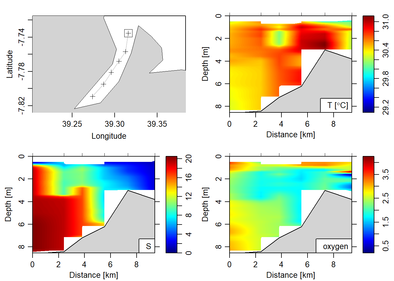

Figure 5: Hydrographic section of Rufiji River

Conclusion

In this post, we have seen the basics of processing CTD data in R with oce package. You have learnt how to import the data, manipulate and proting profiles and section.

Literature Cited

Kelley, D. (2015). Ocedata: Oceanographic datasets for oce. Retrieved from https://CRAN.R-project.org/package=ocedata
Kelley, D., & Richards, C. (2018). Oce: Analysis of oceanographic data. Retrieved from https://CRAN.R-project.org/package=oce
R Core Team. (2018). R: A language and environment for statistical computing. Vienna, Austria: R Foundation for Statistical Computing. Retrieved from https://www.R-project.org/