Seasonal Climatology of temperature and salinity in the WIO region from Argo floats

Import Data

I used delayed mode Argo float data for this post because its profiles have been checked for quality and validated with ship-based in-situ measurements. Some of the variables in the dataset include adjusted temperature, salinity and pressure. Once the dataset was downloaded as netcdf, it was imported into R’s workspace with read.oce(), a function from oce package (Kelley & Richards, 2018). In addition to oce, other packages were loaded into the R to help processing and manipulation of data (Wickham, 2017; Wickham, François, Henry, & Müller, 2018) and for visualize the ouput and mapping (Kelley, 2015; Wickham, 2016; Xie, 2018)

require(tidyverse)
require(oce)
require(ocedata)
require(sf)
require(lubridate)

Because Argo floats have been deployed in the Indian ocean since 2000 and each Argo made several profiles, manual processing the data becomes a daunting task. I use the power of R to iterate the process. The advantge of iteration duplication by automating repeated operations, hence reduce the human error of introducing a bug in the process. Wickham & Grolemund (2016) stated that iteration help to do the same thing to multiple inputs: repeating the same operation on different datasets. Before we iterate the process, the netcidfiles were identified with a ir() function of base R.

# list the netcdf file names in the working directory

argo.file = dir("./argo_profile/",  #relative path of the directory
                recursive = TRUE, # recurse into directory
                pattern = "_prof.nc", # choose the names match this condition
                full.names = TRUE) # get name with its relative path

Tidy the data

Once the list of file names was created, the for() function was used to loop over the netcdf argo files in a sequence order—from the first file to the last one in the working folder. Because the loop has to read the file first and then process the individual profiles in the that particular file, I nested the loop into the outer used latter i and the inner one used latter j. The outer loop (i) read the netcdfiles from working directory, remove bad data in the profiles and align them to the standard depth of five meter interval from the surface to 2000 meters. Then the inner (j) loop manipulate and transformed the profile of each file from oce format to data frame that can easily be handled for further analysis. The main components of loops used to chain the processes in this post are summarized below.

1. The output: argo.ctd = NULL before the looping, I preallocate an empty file to store the iteration output.

2. The sequence: i in 1:length(argo.file) determine what to loop over. Each run of the for loop will assign i to a differrent value from 1:length(argo.file)

3. The body: argo = read.argo(argo.file[i])%>%handleFlags()%>%argoGrid(p = seq(0,2000,5)). This is the code that does the work. It is run repeately, each time with a different value for i.

The outer loop reads the netcdf file with read.argo(), then remove all bad profile data with handleFlags() and then align the profile to standard pressure of five meter interval from the surface to 2000 m deep with argoGrid(p = seq(0,2000,5)). The first iteration will run argo = read.argo(argo.file[1])%>%handleFlags()%>%argoGrid(p = seq(0,2000,5)), the second will run argo = read.argo(argo.file[2])%>%handleFlags()%>%argoGrid(p = seq(0,2000,5)) and so on until to the last file in the argo.file[i]

The inner loops transformed each profile in the argo file into data frame profile = argo.list[[j]]. It then added variables like station name argo = argo.file[i], station = argo.list[[j]][[“station”]]; time the of upload the data time = argo.list[[j]][[“startTime”]]%>%as.Date();longitude longitude longitude = argo.list[[j]][[“longitude”]]; latitude latitude latitude = argo.list[[j]][[“latitude”]]; and computed the density of each measurement in the profile density = argo.list[[j]]%>%swRho(eos = “gsw”). That is lot of talking and may sound difficult and hard to grasp, the code for the procedures above is in the chunk below. It can help you understand better if I might missed something or not explained well. I tried to comment in each step what each code does in the chunk.

# preallocate a file to store processed ctd data
argo.ctd = NULL

# the first section of the loop run with i through the netcdf files
    for (i in 1:length(argo.file)){
        # read the files in sequence
      argo = read.argo(argo.file[i])%>%handleFlags()%>%argoGrid(p = seq(0,2000,5))
        # convert the argo list data into section
      argo.section = argo%>%as.section()
        # convert argo.section into list
      argo.list = argo.section[["station"]]

# the second section of the loop run with j through each argo list created by i
    for (j in 1:length(argo.list)){
      
    profile = argo.list[[j]]@data%>% # get each station profile data
      as.data.frame()%>%          # convert the data into daa frame
            # add variable of argo id, note this use i and not j
      mutate(argo = argo.file[i], 
              #add station variable
             station = argo.list[[j]][["station"]],
              #add date of sampling variable
             time = argo.list[[j]][["startTime"]]%>%as.Date(),
              #add longitude of station variable
             longitude = argo.list[[j]][["longitude"]], 
              #add latitude of station variable
             latitude = argo.list[[j]][["latitude"]], 
              #compute the salinity variable in each station
             density = argo.list[[j]]%>%swRho(eos = "gsw"))%>%
        # convert the data frame into tibble
      as.tibble()%>%
      # drop other variable of no interest
      select(argo, station, time, longitude, latitude,scan, pressure, 
             salinity = salinityAdjusted, temperature = temperatureAdjusted)
    #
    # separate the wmoid into into diferent variables
    profile = profile%>%separate(argo, c(1:7,"wmoid",8), sep = "/")%>%
      # keep the wmoid variable and drop the rest
      select(-c(1:7,9))
    #
    #bind the argo.ctd with the data by rows
    argo.ctd = argo.ctd%>%bind_rows(profile)
  
}
}

Data Frames

You noticed that the process above involved converting netcdf files into tabular data—where a set of values is arranged into columns and rows. In data frame, the rows are observations and columns are variables. In base R, data frame are awesome because most functions for inference, modelling and graphing work well in data frame. Even the set of packages called tidyverse (Wickham, 2017) works in data frame, but prioritized in a modern data frame called tibble. Data frame makes data manipulation and visualization much easier with popular package like ggplot2 (Wickham, 2016) and dplyr (Wickham et al., 2018).

Data frame are unique compared to matrices in R because can hold variables of different flavors like character (Float ID), quantitative data (pressure, salinity, temperature) and qualitative data (monsoon season). Table 1 summarize the number of Argo floats in the area. There are 52 different argo floats that has measured temperature and salinity profiles. This is an interactive table, which allows you to explore in detail the table from your browser by clicking the up and down arrows just after the variable name. You can use this table to understand more about the argo floats in the area. For instance, you can explore which float has the longest measurement period or explore the relationship between the number of profiles and and period for each float.

duration = argo.ctd%>%
  filter(pressure == 10)%>%
  group_by(wmoid)%>%
  summarise(begin = first(time), 
            end = last(time), 
            duration = interval(begin, end)%>%
              as.duration()%>%
              as.numeric("years")%>%
              round(digits = 0), 
            profiles = n())%>%
  arrange(begin)

duration%>% DT::datatable(rownames = FALSE, 
                          colnames = c("Float ID", "Begin Date", "End Date", "Period", "Number of Profiles"),
                          caption = "Table 1: Argo floats in the tropical Indian Ocean region")

Transform

The data from Argo comes as individual netcdf files contain several profiles. Its is not the right format that I needed. I need to transform them into the format that make manipulation and analysis of profile measurement of temperature and salinity across the area much easier. I have already transformed the data in the for loop from the netcdf to data.frame. I will need to create some variable that are needed. the transformation of these dataset include creation of seasonal variable, creation of simple features, creation of grids.

Seasonal Variable

I then added a seasonal column in the existing data frame with a mutate() function. I divided the seaons into northeast (October to March) and southeast monsoon season (April to September).

argo.ctd = argo.ctd%>%
  mutate(season = lubridate::month(time),
         season = replace(season, season %in% c(10:12,1:3), "NE"),
         season = replace(season, season %in% c(4:9), "SE"))

Table interctive table 2 highlight the temperature and salinity and pressure profiles in the Indian Ocean measured with Argo floats number 6902623. This float made it first profile on April, 12, 2015 at longitude 50.17 ^oE ana latitude 0.52 ^oS and made 115 profile until latest prifile records of June 05, 2018. You may notice that there are eight variables—Id, date, longitude, latitude, pressure, temperature, salinity and season. Except the season variable that was tranformed from the date variable, the other seven variable you fetch them from Argo data.

You can interact with this table by searching a specific variable or sort any variable in either ascending or descending order. Xie (2018) developed DT package used to create this interactive table (the chunk below). In short, the chunk speaks like this. In the argo data frame argo.ctd pick observations from argo float with id 6902623; then remove all observations without values; then drop station and scan variables from the data frame; then print all observations from the data frame that met the conditions above as an interactive table. Note that the whole process has been chained with the pipe operator %>% widely referred as then or next

argo.ctd%>%
  filter(wmoid %in% c(6902623))%>%
  na.omit()%>%
  select(-c(station, scan))%>%
  DT::datatable(rownames = FALSE, 
                colnames = c("WMOID","Date","Longitude",
                      "Latitude","Pressure","Salinity","Temperature", "Season"), 
                caption = "Table 2: Argo float information in the tropical Indian Ocean Region") %>%
    DT::formatRound(columns=c("longitude","latitude","salinity", "temperature"), digits=2)

Within the area, Argo floats have measured about 8419 profiles distributed between monsoon seasons. The southeast monsoon has a total of 4191 compared to 4228 profiles during the northeast monsoon season. The distribution of Argo floats within the area is fairly well (Figure 1) during the northeast (Figure 1a) and southeast monsoon season (Figure 1b).

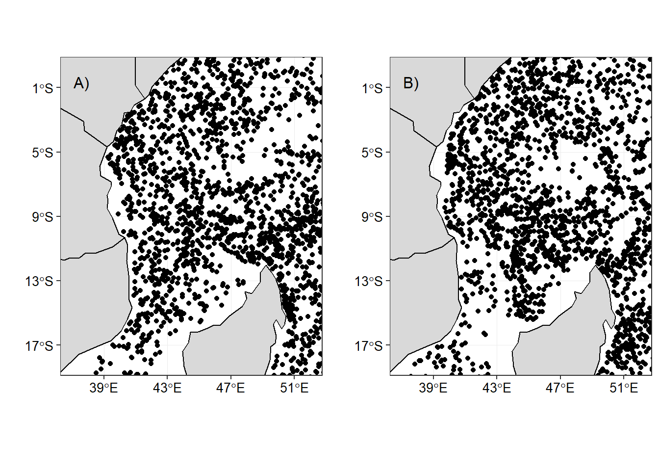
Figure 1: The distribution Argo floats within the tropical Indian Ocean Region during a) northeast and b) southeast monsoon sesons

Create Simple Feature

st_as_sf() function was used to transform a data frame using longitude and latitude information that was used to create a simple featues and define the projection to World Geodetic System (WGS84) as the coordinate sysem.

surface.sf = surface %>% 
  st_as_sf(coords = c("longitude", "latitude")) %>% 
  st_set_crs(4326)

Gridding

To have the homegenous distribution of Argo floats in the region, the area was divided into equal size grids of 900.

grid = surface.sf%>%
  st_make_grid(n = 30)%>%
  # convert sfc to sf
  st_sf()

Populate Grids with Drifter Observations and Median SST

Once the grids were created, I computed the statistics in each grids. The first statistic metric computed was the number of profiles measurements in grids. The second metric was the calculation of median temperature and salinity in each grid. Figure 2a shows the total number of argo floast observations in a grid (Figure 2a) and temperature (Figure 2b) and salinity (Figure 2c) measured near the surface (~10 meter deep)

argo.grid = grid%>%
    # creat an id for each grid
  mutate(id = 1:n(),
  # calculate the index of drifter contained in a grid rectangle       
         contained = lapply(st_contains(st_sf(geometry), 
                                            surface.sf), identity),
  # calculate the number of drifter observations in each grid
         obs = sapply(contained, length),
  # calculate the median temperature in each grid
         temperature = sapply(contained, function(x) {median(surface.sf[x,]$temperature, na.rm = TRUE)}),
  # calculate the median temperature in each grid
         salinity = sapply(contained, function(x) {median(surface.sf[x,]$salinity, na.rm = TRUE)}))

# select some variable of interest
argo.grid = argo.grid%>%select(obs, temperature,salinity)
# summary(sst.grid$sst.median)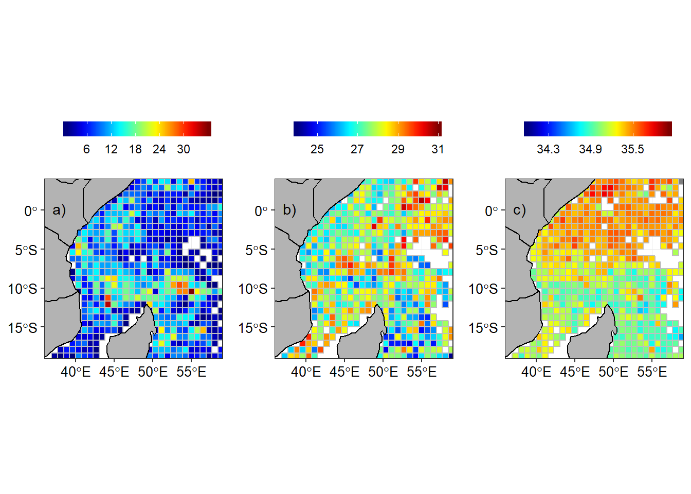

Figure 2: Argo floats in the tropical Indian Ocean a) Number of Argo floats in a grid, b) Temperature and c) Salinity

In order to compare the seasonal climatology distribution of temperature and salinity in the tropical Indian ocean region, the arego floats observation were aligned with the southeast and northeast monsoon season. The regrided spatial distribution of number of argo floats, temperature and salinity are shown for southeast monsoon (Figure 3) and northeast monsoon season (Figure 4).

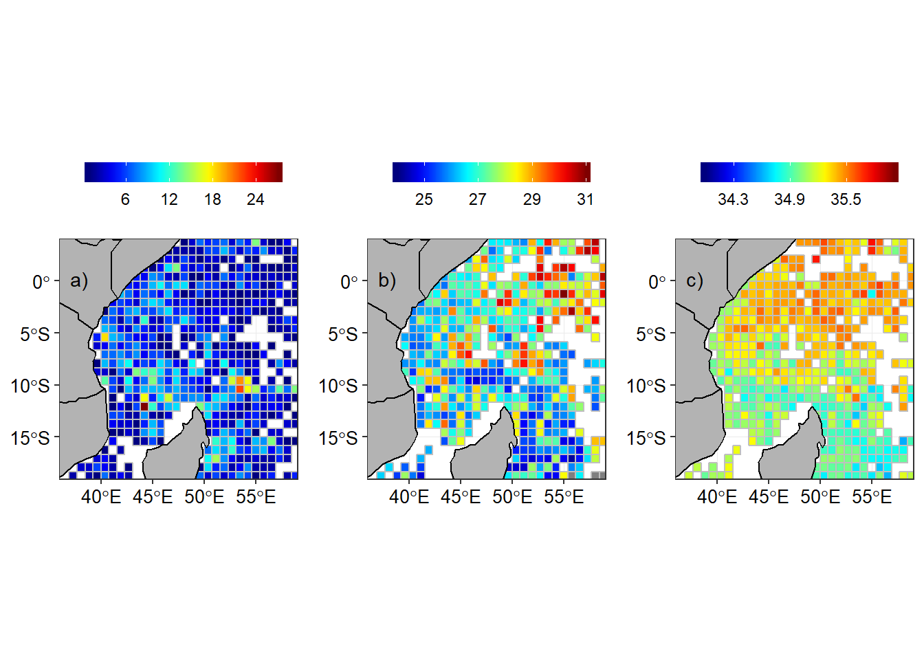
Figure 3: Argo floats in the tropical Indian Ocean during the southeast monsoon season a) Number of Argo floats in a grid, b) Temperature and c) Salinity

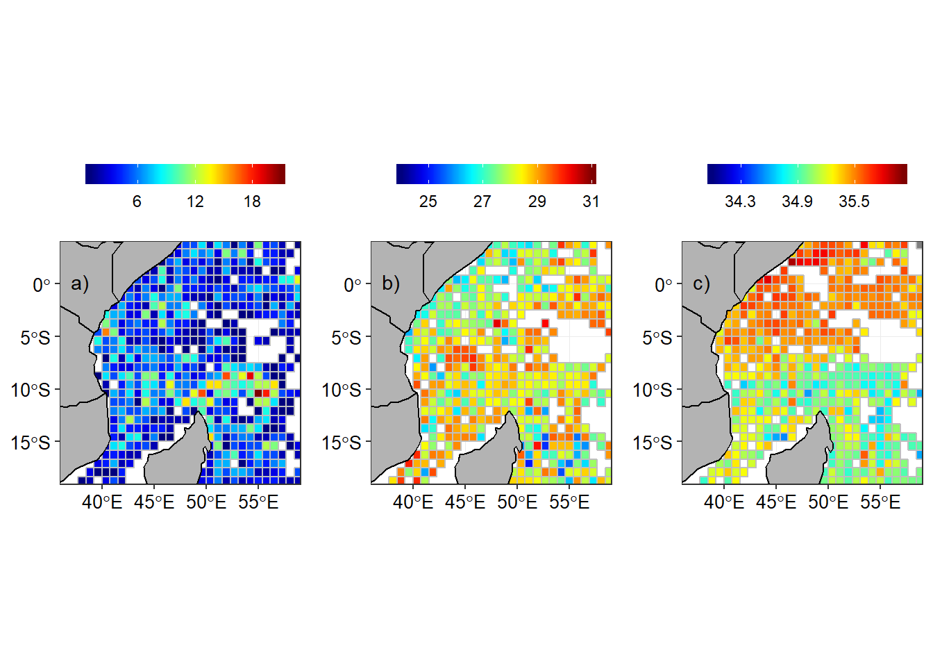
Figure 4: Argo floats in the tropical Indian Ocean during the northeast monsoon season a) Number of Argo floats in a grid, b) Temperature and c) Salinity

References

Carton, X., & L’Hegaret, P. (2011). Mesoscale variability of water masses in the arabian sea as revealed by argo floats. Ocean Science Discussions, 8(3). Journal Article.
Foster, T. D. (1983). The temperature and salinity fine structure of the ocean under the ross ice shelf. Journal of Geophysical Research: Oceans, 88(C4), 2556–2564. Journal Article. https://doi.org/doi:10.1029/JC088iC04p02556
Kelley, D. (2015). Ocedata: Oceanographic datasets for oce. Retrieved from https://CRAN.R-project.org/package=ocedata
Kelley, D., & Richards, C. (2018). Oce: Analysis of oceanographic data. Retrieved from https://CRAN.R-project.org/package=oce
Lauro, F. M., Senstius, S. J., Cullen, J., Neches, R., Jensen, R. M., Brown, M. V., … Grzymski, J. J. (2014). The common oceanographer: Crowdsourcing the collection of oceanographic data. PLOS Biology, 12(9), e1001947. Journal Article. https://doi.org/10.1371/journal.pbio.1001947
Liu, Z., Wu, X., Xu, J., Li, H., Lu, S., Sun, C., & Cao, M. (2017). China argo project: Progress in china argo ocean observations and data applications. Acta Oceanologica Sinica, 36(6), 1–11. Journal Article. https://doi.org/10.1007/s13131-017-1035-x
Roemmich, D., Johnson, G., Riser, S., Davis, R., Gilson, J., Owens, W. B., … Ignaszewski, M. (2009). The argo program: Observing the global oceans with profiling floats. Oceanography, 22(2), 34–43. Journal Article. https://doi.org/10.5670/oceanog.2009.36
Rosell-Fieschi, M. (2014). Ocean velocities as inferred from argo floats: Methodology and applications (Dissertation).
Thadathil, P., Bajish, C. C., Behera, S., & Gopalakrishna, V. V. (2011). Drift in salinity data from argo profiling floats in the sea of japan. Journal of Atmospheric and Oceanic Technology, 29(1), 129–138. Journal Article. https://doi.org/10.1175/JTECH-D-11-00018.1
Vilibić, I., & Mihanović, H. (2013). Observing the bottom density current over a shelf using an argo profiling float. Geophysical Research Letters, 40(5), 910–915. Journal Article. https://doi.org/10.1002/grl.50215
Wickham, H. (2016). Ggplot2: Elegant graphics for data analysis. Springer-Verlag New York. Retrieved from http://ggplot2.org
Wickham, H. (2017). Tidyverse: Easily install and load the ’tidyverse’. Retrieved from https://CRAN.R-project.org/package=tidyverse
Wickham, H., & Grolemund, G. (2016). R for data science: Import, tidy, transform, visualize, and model data. “ O’Reilly Media, Inc.”
Wickham, H., François, R., Henry, L., & Müller, K. (2018). Dplyr: A grammar of data manipulation. Retrieved from https://CRAN.R-project.org/package=dplyr
Xie, Y. (2018). DT: A wrapper of the javascript library ’datatables’. Retrieved from https://CRAN.R-project.org/package=DT