In the post titled Access, Download, Process and VIsualize sea surface height and geostrophic current from AVISO in R posted in my blog on Monday, Apr 15, 2019, I explained how we can download the satellite data like sea surface height from AVISO in R. I illustrate in detail getting the data using xtractomatic package (Mendelssohn 2018). Though xtractomatic package provide functions that allows us to get access to the ERDDAP server and get the data, but one big challenge is that the data comes is array and need an expensive computation process, especially if you deal with gridded data for a long term time series.
Failure of xtractomatic package to provide a tidy format of the gridded data is the reason to write an update post that compliment my previous post. In this post, I will explain an easy way of getting satellite data from ERDAPP server and dowload in tabular form, which is tidy to make use of the power of tidyverse bundles of packages (Wickham 2017). We will use rerddap package (Chamberlain 2017) instead of xtractomatic to accomplish the task. We need to load the package into our session. If you do not have the package in your machine, you can simply install directly from CRAN.
install.packages("rerddap")Then load erddap and tidyverse packages that we are going to use in this post
require(rerddap)
require(tidyverse)
The ERDDAP server has thousands of gridded and table dataset, and can be overwheliming to look at these dataset manually. The rerddap package has a ed_search function that allows us to query the server with specific type of keywords. For instance I am interested with all one day composite chlorophyll a dataset with global coverage. I can simply parse the argument ed_search(query = "MODIS Chlorophyll-a Global 1 Day") and get the list of all dataset that meet those criteria.
whichchl = ed_search(query = "MODIS Chlorophyll-a Global 1 Day")The list of dataset has a title and dataset_id. The title provide a glimpse of the dataset and the dataset_id is the key entry for which to download the data. I picked the monthly composite chlorophyll dataset erdMH1chlamday and used the info function from rerdapp package to obtain the internal information of the dataset;
info("erdMH1chlamday")<ERDDAP info> erdMH1chlamday
Base URL: https://upwell.pfeg.noaa.gov/erddap/
Dimensions (range):
time: (2003-01-16T00:00:00Z, 2020-08-16T00:00:00Z)
latitude: (-89.97918, 89.97916)
longitude: (-179.9792, 179.9792)
Variables:
chlorophyll:
Units: mg m^-3 # info("erdMH1chla1day")The erdMH1chlamday function when parsed to the info function provide as with details like the variable names, the geographical extent in longitude and latitude and the time bound of the dataset. This information is useful as they guide us to select only the data available within the geographical extent and time bounds. If we define the extent and bound outside those in the dataset, we will get an error message.
To download the gridded data, we use griddap function and define the latitude, longitude and time bounds of the data we wish to download. For instance the chunk below shows that I am interested with all monthly values of chlorophyll from 4 km MODIS dataset that are within longitude metR::LonLabel(-76.30499) and metR::LonLabel(-77.03618) and latitude metR::LatLabel(34.248) and metR::LatLabel(34.3516) and must be acquired between 2009-09-30 and 2013-09-30. Since I want tidy data, I parse a fmt = "csv", which will download and arrange the data in tabular form.
chla = griddap("erdMH1chlamday",
                      latitude =  c(34.248, 34.3516),
                      longitude = c(-76.30499, -77.03618),
                      time = c("2009-09-30", "2013-09-30"),
                      fmt = "csv")
Once the data is downloaded, I can use amutate function from dplyr package (Wickham et al. 2018) to reformat the date into the right format using a as_date() from lubridate package (Grolemund and Wickham 2011). A sample tibble file of the dataset is presented below, which show the first and last three observations.
chla = chla %>%
  mutate(time = lubridate::as_date(time))

## Visualize the head and tail of the dataset
chla %>% FSA::headtail() %>% as_tibble()
# A tibble: 6 x 4
time latitude longitude chlorophyll
<date> <dbl> <dbl> <dbl>
1 2009-09-16 34.4 -77.0 0.316
2 2009-09-16 34.4 -77.0 0.324
3 2009-09-16 34.4 -76.9 0.318
4 2013-09-16 34.2 -76.4 0.274
5 2013-09-16 34.2 -76.4 0.274
6 2013-09-16 34.2 -76.3 0.271chla %>%
filter(time <= "2009-12-16") %>%
ggplot(aes(x = longitude, y = latitude)) +
geom_tile(aes(fill = chlorophyll))+
scale_fill_gradientn(colours = mycolor, trans = scales::log10_trans())+
facet_wrap(~time)And figure 1 created with ggplot2 (Wickham 2016) and metR (Campitelli 2019) packages gives a visual appeal of how chlorophyll concentration in this area vary toward the end of the year 2009.
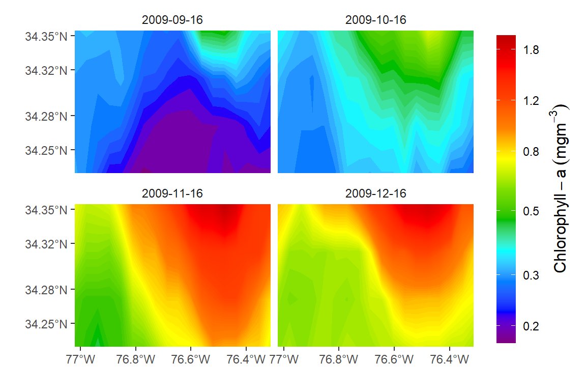
Figure 1: Chlorophyll-a concentration of months for the last quarter of 2009
References
Campitelli, Elio. 2019. MetR: Tools for Easier Analysis of Meteorological Fields. https://CRAN.R-project.org/package=metR.
Chamberlain, Scott. 2017. Rerddap: General Purpose Client for ’Erddap’ Servers. https://CRAN.R-project.org/package=rerddap.
Grolemund, Garrett, and Hadley Wickham. 2011. “Dates and Times Made Easy with lubridate.” Journal of Statistical Software 40 (3): 1–25. http://www.jstatsoft.org/v40/i03/.
Mendelssohn, Roy. 2018. Xtractomatic: Accessing Environmental Data from Erd’s Erddap Server. https://CRAN.R-project.org/package=xtractomatic.
Wickham, Hadley. 2016. Ggplot2: Elegant Graphics for Data Analysis. Springer-Verlag New York. http://ggplot2.org.
———. 2017. Tidyverse: Easily Install and Load the ’Tidyverse’. https://CRAN.R-project.org/package=tidyverse.
Wickham, Hadley, Romain François, Lionel Henry, and Kirill Müller. 2018. Dplyr: A Grammar of Data Manipulation. https://CRAN.R-project.org/package=dplyr.