The study of sea surface temperature (SST) is one of the cornerstone of oceanography. It has applications not only in physics (Bader & Latif, 2003), chemistry (Corrège, 2006) and the earth’s sciences, but in subjects as diverse as biology and economics. SST plays an important role in our quantitative understanding of coastal habitats and species distribution in our global oceans (Grémillet et al., 2008; Müller-Karger, Walsh, Evans, & Meyers, 1991).
Minnett et al. (2004) clearly state that until the launch of The Moderate Resolution Imaging Spectroradiometer (MODIS) early 2000s, oceanographers were unable to obtain information of SST at fairly resolution . Since July 2002, MODIS provides SST for all global ocean at 4 km spatial resolution every 3 days (Chen et al., 2011). MODIS products enable scientists to address some issues that were impossible without the satellite derived products.
We know much about the satellite derived SST products from MODIS, but little attention has been placed on the SST gathered in-stu with drifters. Therefore, this post goal is to introduce some fundamentals techniques on how to process SST data from Global Drifter Program. But important, I will trail the processes in this post using R—a free and open source programming language R Core Team (2018)]. I loaded four packages—tidyverse developed (Wickham, 2017), lubridate (Grolemund & Wickham, 2011), kableExra (Zhu, 2018) and sf (Pebesma, 2018) but I also used cowplot package for combining figures (Wilke, 2018).
require(tidyverse)
require(lubridate)
require(sf)
require(kableExtra)
Drifter processing
Figure 1 summarise the main analytical step used in this post. This data model is modified from Wickham & Grolemund (2016). Thre model consists of mainly three steps. The first, the dataset was downloade from NOAA as ascii file. Second, the dataset was imported in R using the dplyr’s read_table() function. Third, once the dataset was in the workspace, it was manipulated and transformed. These dataset has twelve variables, I cleaned the dataset by removing some variables not needed for this post. I kept the common id, longitude, latitude, year, month, day and sst variables. Fourth, the observations were later grouped based on monsoon seasons. All drifter observations recorded between April and September fell into southeast monsoon season (SE). And those between October and March fell in the northeast (NE) monsoon season. Table 1 show drifter observation after being procesed.
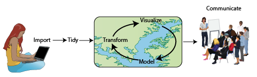
Figure 1: The data analysis model
# read the file from the local drive
drifter = read_table2("./drifters.txt",
                      col_names = FALSE, comment = "#")%>%
  select(id = 1, lon = 2, lat = 3, drogue =4, u = 5, v = 6,
         sst = 7, year = 8, month = 9, day = 10, hour = 11)

drifter = drifter%>%
  mutate(date = make_date(year, month, day),
         velocity = sqrt(u^2 + v^2),
    # make season variable
         season = month,
    # convert months into seasons
         season = replace(season,season %in% c(10,11,12,1,2,3), "NE"),
         season = replace(season, season %in% c(4:9), "SE"))%>%
    # select variables of interest and drop others
select(date, season,id,lon,lat, u,v,velocity,sst)| Date | Season | Longitude | Latitude | Drifter ID | SST |
|---|---|---|---|---|---|
| 2007-06-06 | SE | 47.95 | -6.82 | 62198 | 27.95 |
| 1996-01-22 | NE | 45.47 | -6.73 | 9421923 | NaN |
| 2014-05-06 | SE | 41.46 | -7.47 | 109290 | 28.74 |
| 2007-01-22 | NE | 50.95 | -14.34 | 63904 | 29.36 |
| 2008-12-10 | NE | 50.74 | -8.48 | 70864 | 28.85 |
| 2014-07-12 | SE | 43.69 | -9.70 | 126952 | 25.73 |
| 1986-06-20 | SE | 41.95 | -10.93 | 8603091 | 26.08 |
| 2006-10-08 | NE | 43.03 | -4.93 | 62549 | 26.57 |
| 2008-08-14 | SE | 41.80 | -8.39 | 46036 | 24.84 |
| 2001-04-03 | SE | 47.61 | -11.66 | 28941 | 28.80 |
| 2000-11-05 | NE | 51.92 | -9.23 | 18735 | NaN |
| 1993-11-04 | NE | 40.27 | -3.38 | 9217262 | NaN |
| 2013-07-14 | SE | 46.81 | -9.32 | 114571 | 24.95 |
| 1997-12-04 | NE | 43.60 | -8.49 | 9619176 | NaN |
| 2000-07-26 | SE | 42.41 | -12.47 | 17444 | 25.07 |
| 2014-10-27 | NE | 45.09 | -11.86 | 101833 | 27.29 |
| 2013-05-23 | SE | 40.63 | -9.14 | 109373 | 27.09 |
| 2000-07-25 | SE | 42.30 | -12.27 | 17444 | 25.21 |
| 1996-10-16 | NE | 42.42 | -13.88 | 9423511 | 27.10 |
| 1999-09-02 | SE | 42.01 | -1.18 | 9730554 | NaN |
Create Simple Feature
Because this post deals with spatial analysis, I converted the drifter dataset from data frame to simple feature and assign the dataset with WGS84 as the coordinate sysem.
drifter.sst = drifter%>%select(-c(u,v,velocity))

drifter.sst.sf = drifter.sst%>%
  st_as_sf(coords = c("lon", "lat"))%>%
  st_set_crs(4326)
Divide the Area into Grids
Because drifter observations are inhomogenous distributed within the Tropical Indian Ocean region, to obtain homogenous distribution, I divided the region into 900 grids covering the entire area.
# creat a grids of the area
grid = drifter.sst.sf%>%st_make_grid(n = 30)
Populate Grids with Drifter Observations and Median SST
Once the grids were created, I computed the statistics in each grids. The first statistic metric computed was the number of observations in grids . Then the second metric was the calculation of median SST in a grid.
Visualization
The Western Indian Ocean Region is fairly crossed with Lagrangian drifter observations (Figure 2a). Grids with drifters above 300 are found North the Madascar Island and extend to the west of the Island toward the East African coast. The largest part of the area has grids with less than 100 drifter per grid. The climatology sea surface temperature from drifters range between 25 oC and 30oC with mean tempeature of 27.80 oC. The warmest water lies between latitude 4 to 10 oS (Figure 2b). This warmest region lies in the southern gyres as shown in the previous post.
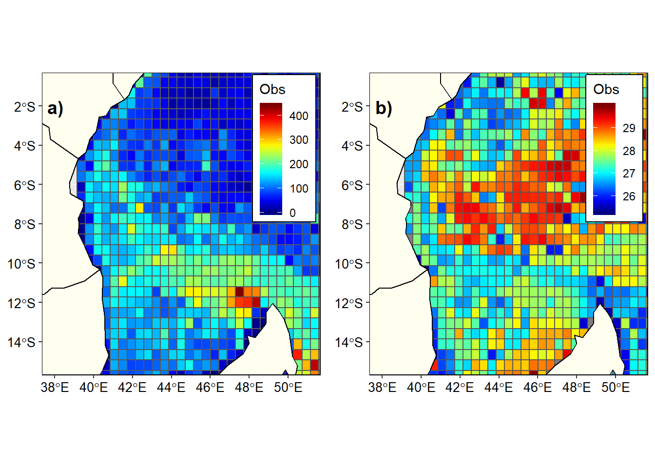
Figure 2: Climatology a)Total number of drifters and b) the median SST in the Tropical Indian Ocean region
Seasonal Variation
Figure 3 show the seasonal median sea surface current within the tropical Indian ocean region. Like other studies, drifter observations reveals the northeast season has fairly higher sea surface temperature compared to the southeast monsoon season (Figure 3).
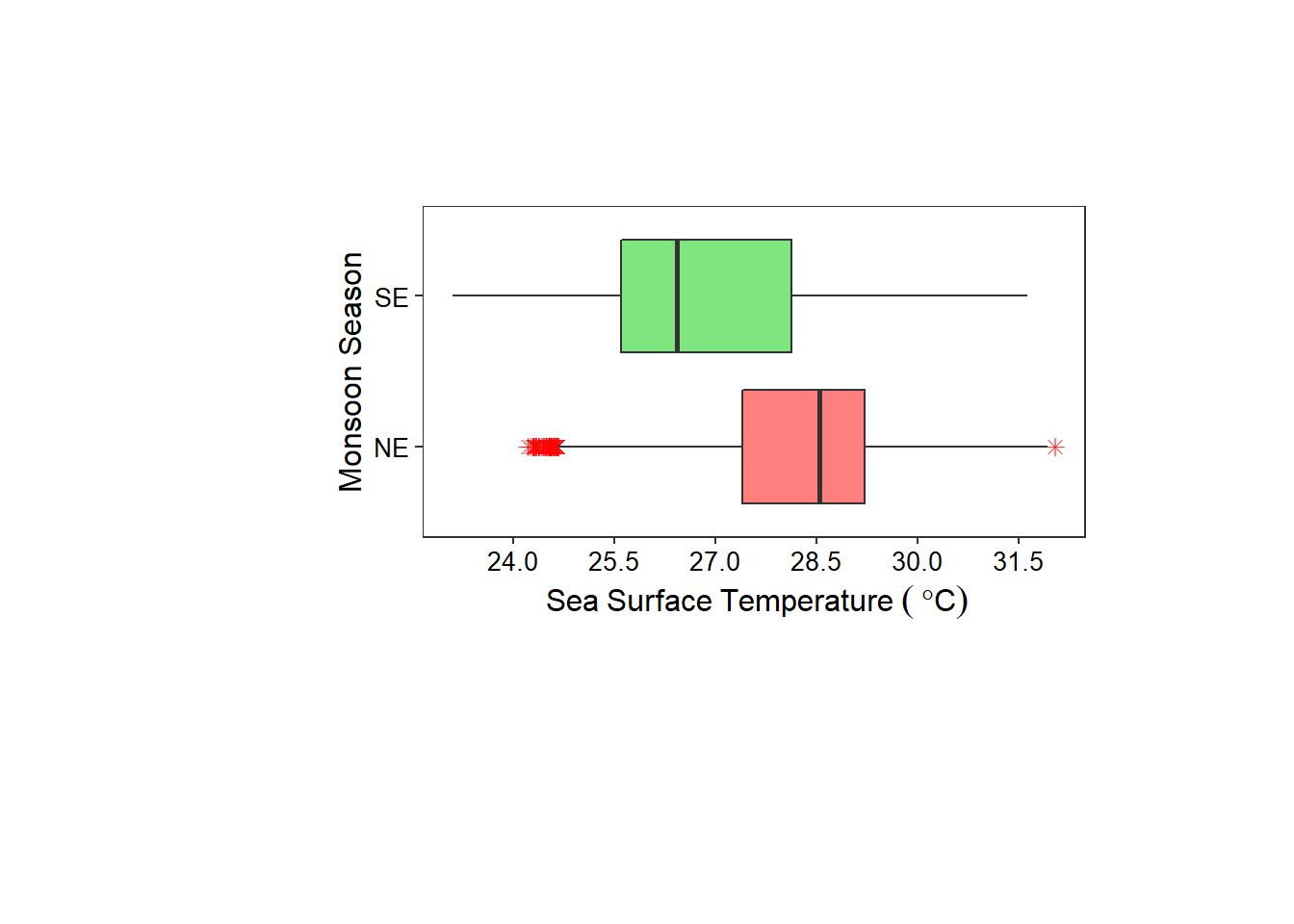
Figure 3: The sea surface current during the northeast (NE) and southeast (SE) monsoon season
Southeast Monsoon Period
All drifters crossed the region between April and September were combined to form the southeast monsoon. The pattern of drifters distribution during the climatology southeast monsoon period (Figure 4) matches closely to those in figure 2a, though the number is less. However, the climatology sea surface temperature during the southeast monsoon period does not show clear patter, even the dongue of warm water is not visibl (figure 4b)e. This is because both the East African Coastal Current and Somali CUrrent both flow northward during the southease monsoon and weaken cyclonic flow around the equator leading to disappearing of southern gyre.
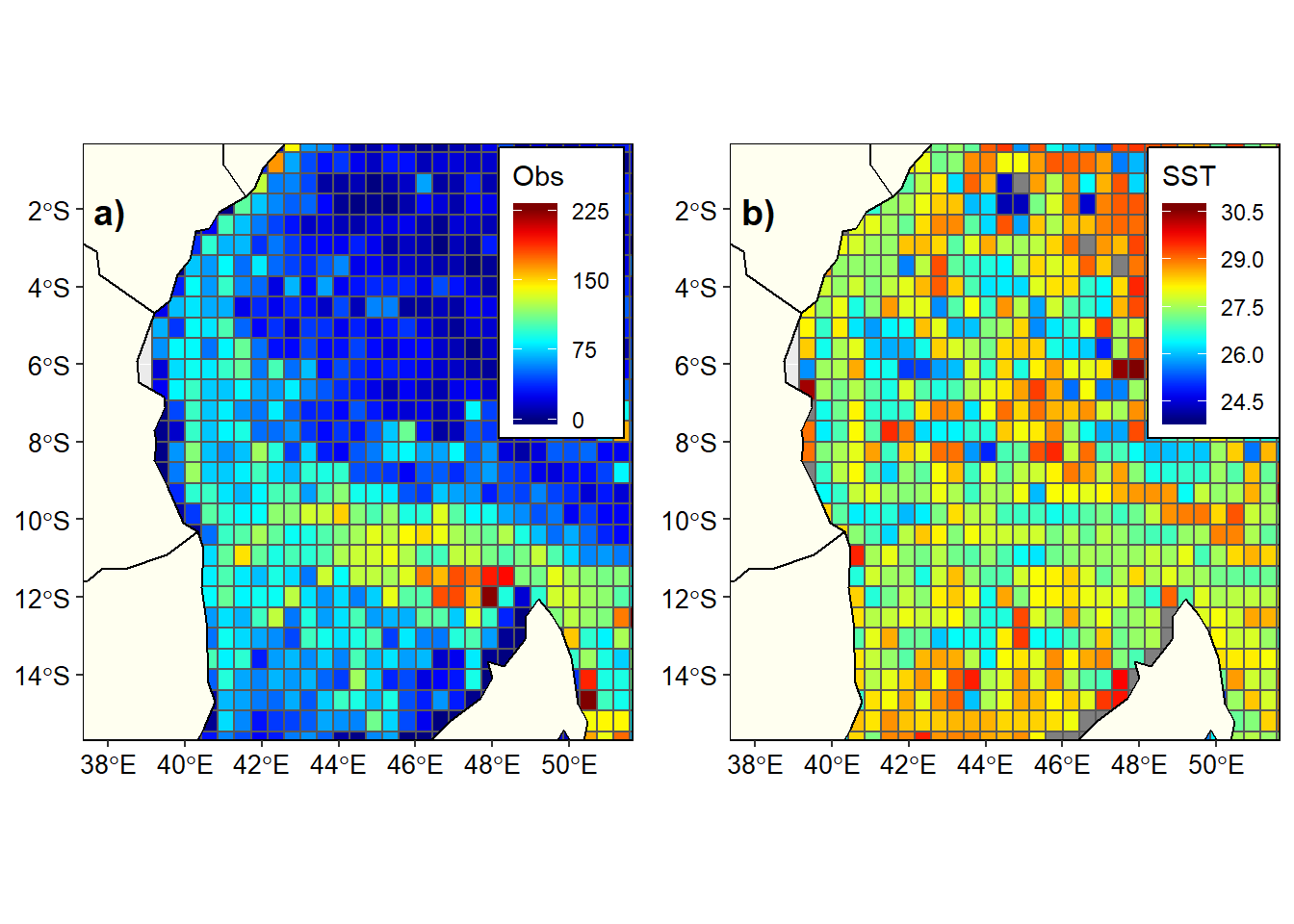
Figure 4: Climatology drifter observation during the southeast monsoon season. a)Total number of drifters and b) the median SST in a grid
Northeast monsoon Period
Unlike the southeast, the climatology northeast period had few drifters throughout the region. Most of the area had drifters below 75 except some few grids west of north Madagascar Island (Figure 5a). Yet although northeast season has few drifter but the pattern of areas with large number of drifter is similar to those in figure 2a and 4. We also notice that the the pattern of sea surface temperature during the northeast (Figure 5b) differs with the southeast season (Figure 4b). The northeast monsoon is associated with warmest water above 30 oC along the coastal areas.
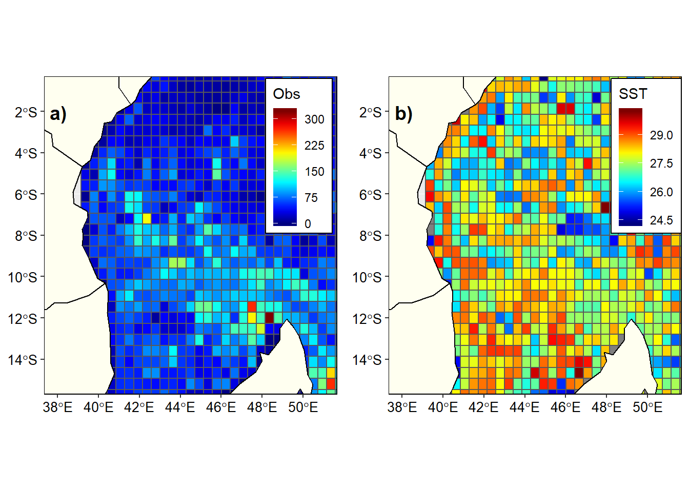
Figure 5: Climatology drifter observation during the northeast monsoon season. a)Total number of drifters and b) the median SST in a grid
Conclusion
As we have seen there are more drifters during the southeast monsoon (Figure 4a) than the northeast monsoon (Figure 5a). Drifter reveals the presence of warm temperature southern gyre (Figure 2a). Threfore, drifter observation from Global Drifter Program provides reliable in-situ data that can be used to validate and calibrate satellite-derived sea surface temperatue in the tropical Indian Ocean Region.
References
Bader, J., & Latif, M. (2003). The impact of decadal-scale indian ocean sea surface temperature anomalies on sahelian rainfall and the north atlantic oscillation. Geophysical Research Letters, 30(22).
Chen, Y., Randerson, J. T., Morton, D. C., DeFries, R. S., Collatz, G. J., Kasibhatla, P. S., … Marlier, M. E. (2011). Forecasting fire season severity in south america using sea surface temperature anomalies. Science, 334(6057), 787–791.
Corrège, T. (2006). Sea surface temperature and salinity reconstruction from coral geochemical tracers. Palaeogeography, Palaeoclimatology, Palaeoecology, 232(2-4), 408–428.
Grémillet, D., Lewis, S., Drapeau, L., Der Lingen, C. D. van, Huggett, J. A., Coetzee, J. C., … Ryan, P. G. (2008). Spatial match–mismatch in the benguela upwelling zone: Should we expect chlorophyll and sea-surface temperature to predict marine predator distributions? Journal of Applied Ecology, 45(2), 610–621.
Grolemund, G., & Wickham, H. (2011). Dates and times made easy with lubridate. Journal of Statistical Software, 40(3), 1–25. Retrieved from http://www.jstatsoft.org/v40/i03/
Minnett, P. J., Brown, O. B., Evans, R. H., Key, E. L., Kearns, E. J., Kilpatrick, K., … Szczodrak, G. (2004). Sea-surface temperature measurements from the moderate-resolution imaging spectroradiometer (modis) on aqua and terra. In Geoscience and remote sensing symposium, 2004. igarss’04. proceedings. 2004 ieee international (Vol. 7, pp. 4576–4579). Ieee.
Müller-Karger, F. E., Walsh, J. J., Evans, R. H., & Meyers, M. B. (1991). On the seasonal phytoplankton concentration and sea surface temperature cycles of the gulf of mexico as determined by satellites. Journal of Geophysical Research: Oceans, 96(C7), 12645–12665.
Pebesma, E. (2018). Sf: Simple features for r. Retrieved from https://CRAN.R-project.org/package=sf
R Core Team. (2018). R: A language and environment for statistical computing. Vienna, Austria: R Foundation for Statistical Computing. Retrieved from https://www.R-project.org/
Wickham, H. (2017). Tidyverse: Easily install and load the ’tidyverse’. Retrieved from https://CRAN.R-project.org/package=tidyverse
Wickham, H., & Grolemund, G. (2016). R for data science: Import, tidy, transform, visualize, and model data. “ O’Reilly Media, Inc.”
Wilke, C. O. (2018). Cowplot: Streamlined plot theme and plot annotations for ’ggplot2’. Retrieved from https://CRAN.R-project.org/package=cowplot
Zhu, H. (2018). KableExtra: Construct complex table with ’kable’ and pipe syntax. Retrieved from https://CRAN.R-project.org/package=kableExtra