Introduction
In the previous post I showed how to track the East African Coastal Current using trajectories od drifters. In this post, we dive deeper, focusing on creating grids and fill them with number of drifter the median surface current and present them in form of maps. The goal of this routine is to illustrate how to process drifter data in R using tidyverse and other packages.
Needed Packages
We need to load some packages into R that are used to process the data. The chunk below show the list of packages I selected that I will use to import the data, manipulate, transform and last presented the results in form of maps. One of the package is the tidyverse, which loads five other packages — ggplot2, tibble, tidyr, readr, purrr, and dplyr packages. These are considered to be the core of the tidyverse because are mostly used in almost every analysis. In addition to tidyverse, I used Other packages likesf1 package to handles well spatial data, lubridate2 for date and time manipulation and kableExtra3 for stylish reporting of data in tabular forms.
require(tidyverse)
require(lubridate)
require(kableExtra)
require(sf)
Data Manipulation
I obtained drifter observations as rectangular data. This means a dataset organized in such way that column are associated with variables and rows are associated with observations. Wickham term this type of data arrangement as tidy. I used used the dplyr’s function read_table2() to import the data into R’s workspace. read_table2() is designed to read the type of textual data where each column is separated by one (or more) columns of space.
## load the dataset
drifter = read_table2("./drifters.txt", comment = "#",
                     col_names = FALSE)
Once the data was in the workspace, I found the data comes without column names and it also contains columns with empty cells. In this case, the first process I did is to rename the variables with appropriate names using the dpyr’s function rename().
drifter = drifter%>%select(id = X1, lon = X2, lat = X3,
                           drogue = X4, u = X5, v = X6,
                           sst = X7, year = X8, month = X9,
                           day = X10, hour = X11)
Because the monsoon season affects the surface current circulation in the tropical Indian Ocean Region, I create a seasonal variable from the month variable and computed the surface current velocity based on the equation (1).
\[ \begin{equation} Velocity \:(ms^{-1})\:=\: \sqrt{(U^2+V^2)} \tag{1} \end{equation} \]
Creating Simple features
I used sf package that implements a formal standard called “Simple Features” that specifies a storage and access model of spatial geometries (point, line, polygon). A feature geometry is called simple when it consists of points connected by straight line pieces, and does not intersect itself. Using the unique identification number of drifters. A sf’s function st_as_sf() was used to create point features using longitude and latitude information of drifter dataset and then set the Coordinate system to World Geodetic System of 1984 (WGS84).
## create simple features
drifter.sf = drifter%>%
  select(season, id, lon,lat ,u,v)%>%
  mutate(velocity = sqrt(u^2 + v^2))%>%
  st_as_sf(coords = c("lon", "lat"))%>%
  st_set_crs(4326)
Create rectangular grids
Because I wanted to have the distribution of drifter data in equally spaced grid, I first created gridded polygons with the sf’s function st_make_grid() and opted for 1600 grids (40 \(\:\times \:\) 40) (Figure 1). The grid generated was simple feature geometry list-column (sfc) format, which prevent computation. To allow further analysis and computation, the sfc gridded file was transformed to sf using st_sf() function.
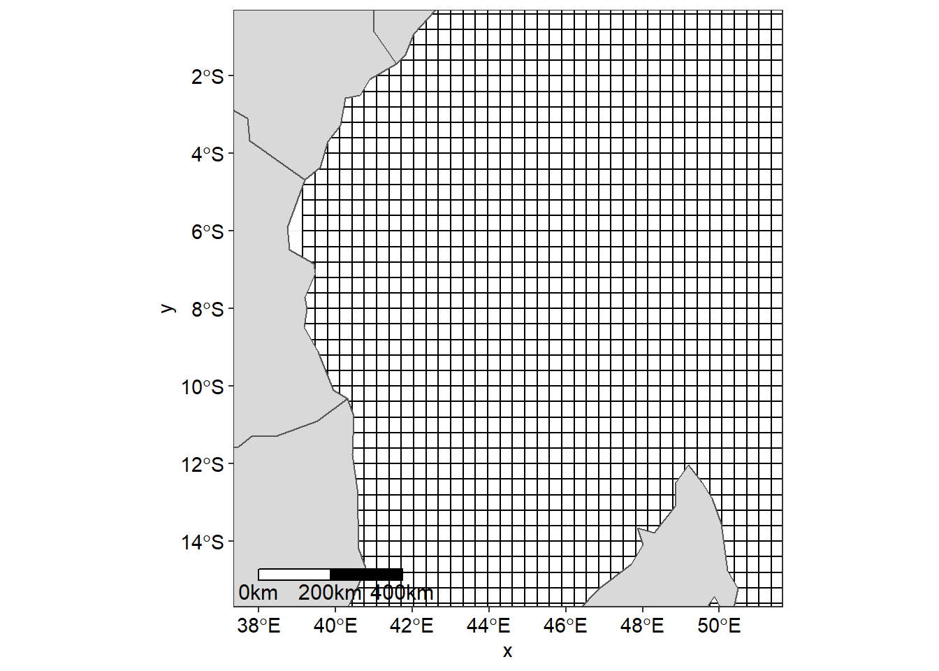
Figure 1: The Tropical Indian Ocean Area has been sliced into equal spaced grids
Filling the grids with values
Once the gridding process was complete, the total number of drifter in each grid was calculated. This approach has been used previously and successfully with sparsely sampled, inhomogenous oceanographic data sets4. The total number of observations within a grid were calculate using equation (2). Once the number of observations were determined, only grids with more than four observation of drifters were selected to calculate the median zonal component in equation (3), the median meridional component in equation (4) and the median median velocity in equation (5) for each grid.
\[ \begin{equation} \tau_i \:=\:\sum_{i=n}^{n} x_{i} \tag{2} \end{equation} \]
\[ \begin{equation} \varphi = \frac{\sum(\varphi_i + \varphi_{i+1} + \varphi_{i+3} + \varphi_{i+ \cdots n})}{\sum_{i = n}N} \tag{3} \end{equation} \]
\[ \begin{equation} \lambda = \frac{\sum(\lambda_i + \lambda_{i+1} + \lambda_{i+3} + \lambda_{i+ \cdots n})}{\sum_{i = n}N} \tag{4} \end{equation} \]
\[ \begin{equation} \upsilon = \frac{\sum(\upsilon_i + \upsilon_{i+1} + \upsilon_{i+3} + \upsilon_{i+ \cdots n})}{\sum_{i = n}N} \tag{5} \end{equation} \]
Results
The information of binned drifter are shown in table 1. The centroid are the longitude and latitude position extracted from the center of each grid. These information include number of observations, zonal, meridional meridional values and computed velocity for each grid. The number of drifter in a grid (Table 1) was used to map the distribution of drifters observations within the region. The distribution of surface current was also mapped using the velocity variable (Table 1)| Longitude | Latitude | in a Grid | Zonal | Meridional | Velocity |
|---|---|---|---|---|---|
| 47.34 | -13.4 | 102 | 0.05 | -0.05 | 0.39 |
| 44.45 | -11.0 | 119 | -0.63 | -0.04 | 0.73 |
| 51.52 | -4.2 | 44 | 0.16 | 0.29 | 0.46 |
| 42.84 | -7.0 | 73 | -0.11 | 0.07 | 0.25 |
| 39.63 | -5.4 | 35 | -0.32 | 0.85 | 0.93 |
| 40.27 | -4.2 | 80 | 0.29 | 0.88 | 0.96 |
| 43.49 | -12.2 | 36 | -0.16 | -0.29 | 0.58 |
| 41.56 | -9.8 | 62 | -0.35 | 0.06 | 0.38 |
| 41.88 | -0.2 | NA | NA | NA | NA |
| 43.81 | -1.0 | 26 | -0.09 | 0.00 | 0.14 |
| 49.59 | -1.8 | 29 | -0.26 | -0.20 | 0.46 |
| 44.13 | -9.0 | 103 | -0.17 | -0.03 | 0.27 |
Figure 2 reveals the spatial distribution of drifter observations vary across the tropical Indian Ocean region. A large proportion of the area has less than 100 drifter observation except the west side of Madagascar and Comoros Islands that receive more than 150 observations (Figure 2)
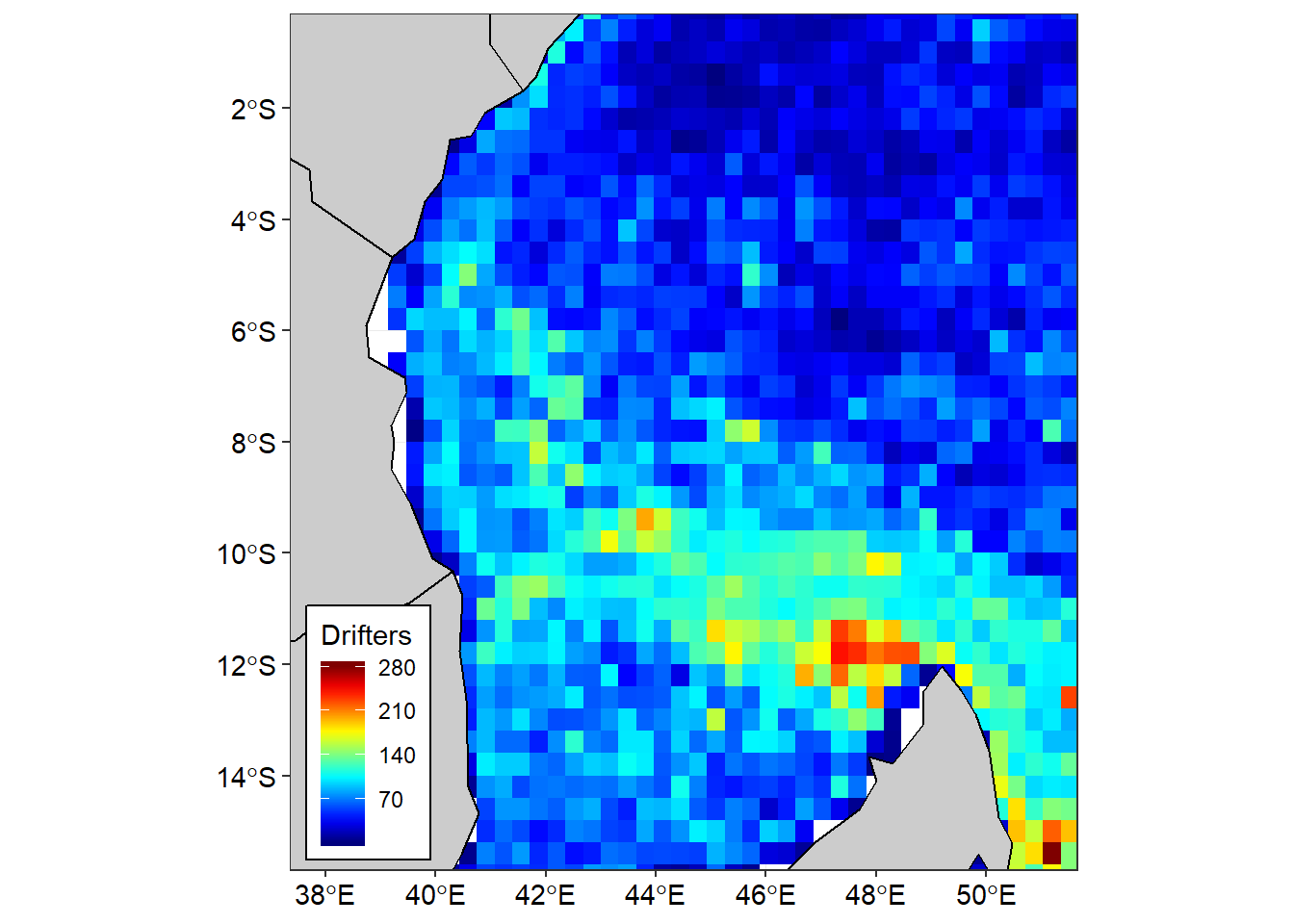
Figure 2: Cumulative drifter observations (Number of drifter per grid) in the Tropical Indian Ocean Region
The surface current vectors in Figure 3 was compiled from climatological drifter observations from the Global Drifter Program. In this figure the surface circulation agrees quite well with results found by Swallow et al,, (1991)5.
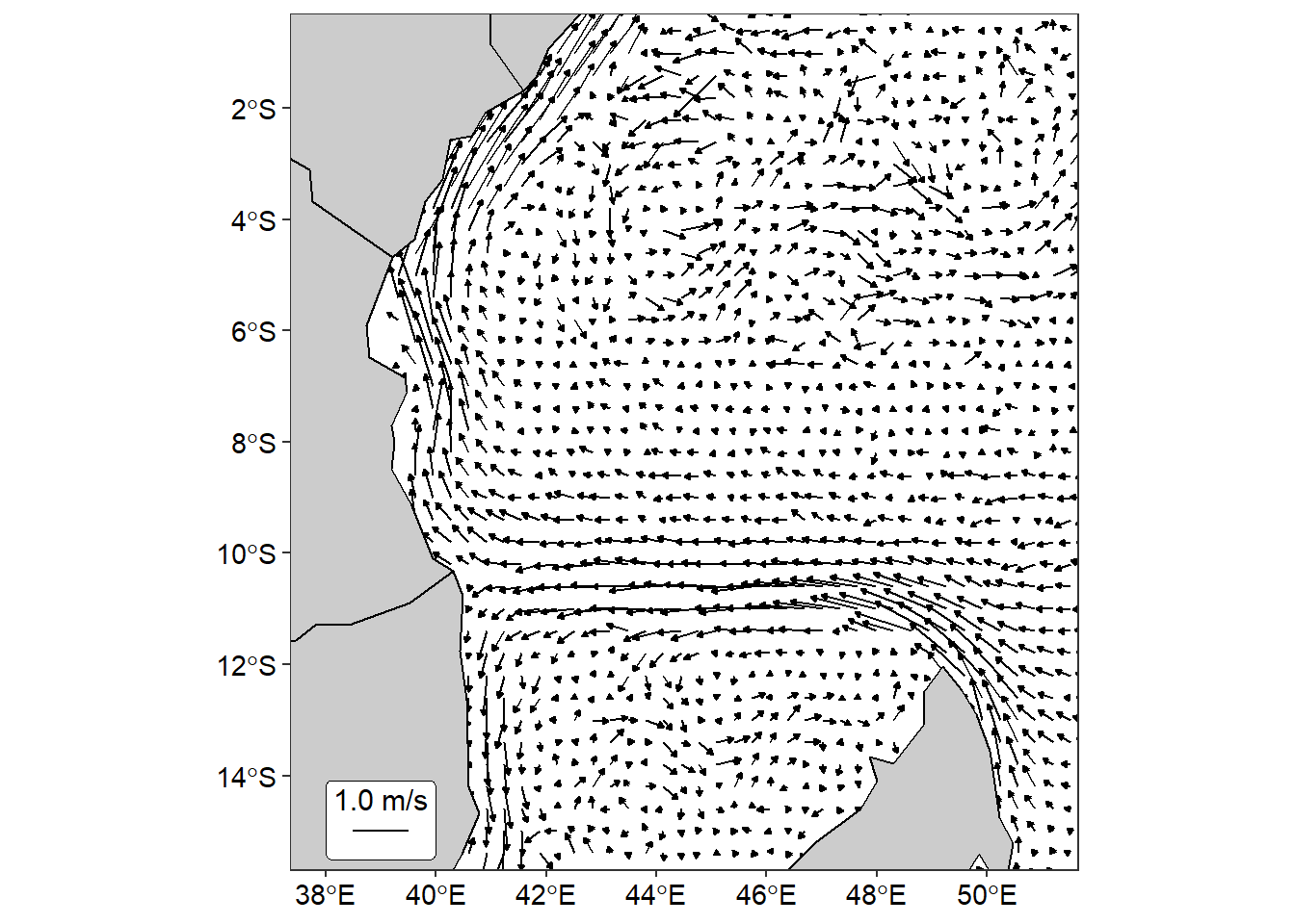
Figure 3: Climatological mean of near-surface currents derived from satellite-tracked drifter trajectories
When these vectors are superimposed with surface current velocity, a clear pattern of surface circulation is revealed (Figure 4). The features of prominent regional surface current are visible in the drifter-derived velocity fields like the East African Coastal Current and the South Equatorial Current, particularly where the currents are strong. Drifter also shows the split of the south equatorial current into the north flowing East African Coastal Current and south flowing into the Mozambique Channel at about 11 \({^\circ}\)S (Figure 4). The surface velocity of EACC reaches a maximum of 1.5ms-1, which is the highest when compared to the SEC and the Mozambique Channel (Figure 4). Although not clear, a southern gyres is also apparent from drifters.
Figure 3 and 4 further reveal the strength of EACC that increase in median velocity northward from 7.5 \({^\circ}\)S off the Mafia Island and path off Ungjua island, but in Pemba Island it path in both side of the island and reaches its full speed of about1.5 ms-1 along the coastal water of Kenya. The westward flow feeding into the EACC appears to be mainly, but not entirely, concentrated between latitudes 9 \({^\circ}\)S and 11\({^\circ}\)S (Figure 4).
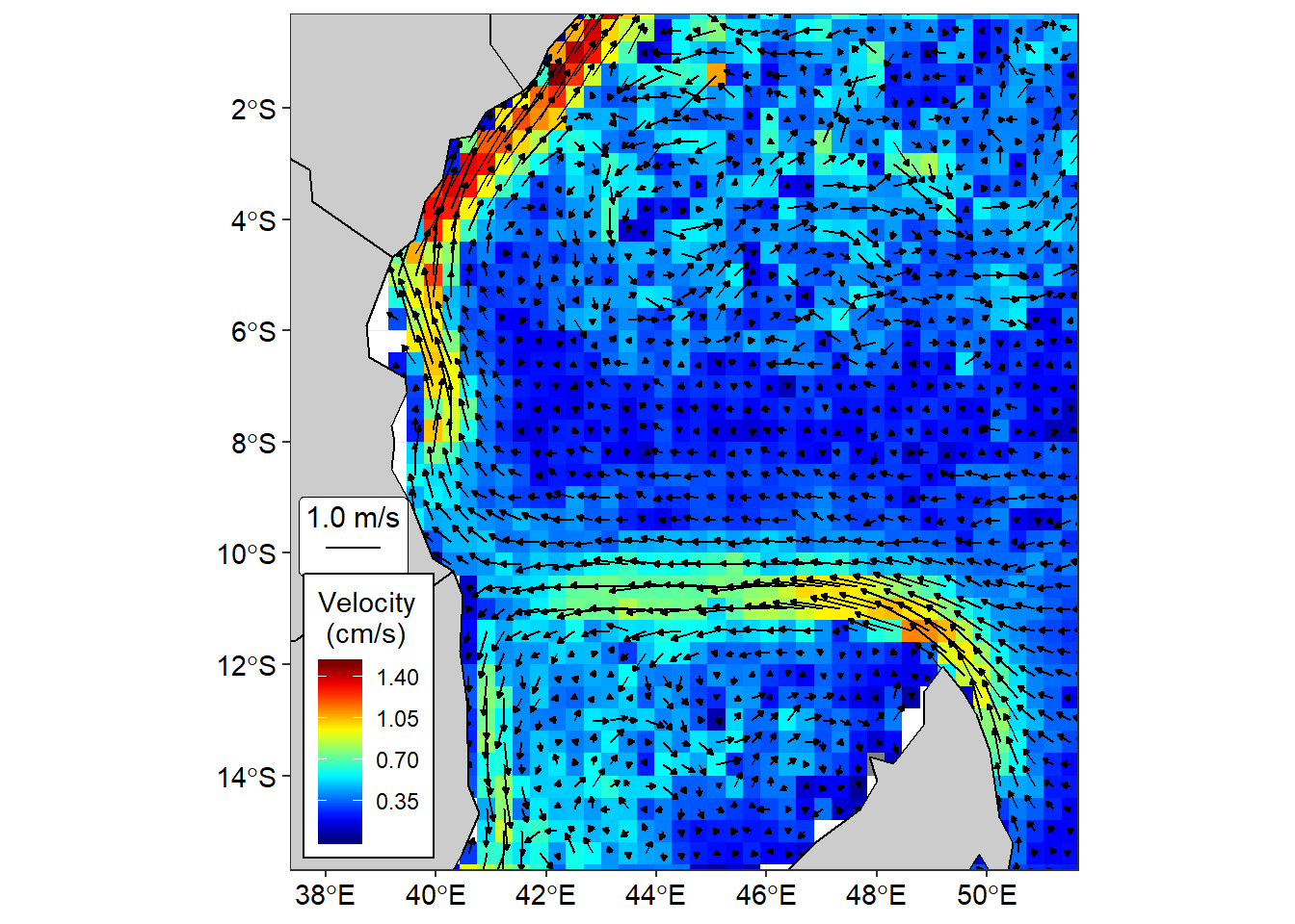
Figure 4: Climatological median of near-surface currents vector overlaid on surface current velocity
Conclusion
Drifters from Global Drifter Program captured well the surface circulation in the tropical Indian Ocean Region. They revealed well the surface circulation in Figures 3 and 4. Furthermore, drifters clearly show the climatological median of surface current in southern end of the EACC is close to 11 \(^{\circ}\)S.
Cited References
Edzer Pebesma (2018). sf: Simple Features for R. R package version 0.6-3. https://CRAN.R-project.org/package=sf↩
Garrett Grolemund, Hadley Wickham (2011). Dates and Times Made Easy with lubridate. Journal of Statistical Software, 40(3), 1-25. URL http://www.jstatsoft.org/v40/i03/.↩
Hao Zhu (2018). kableExtra: Construct Complex Table with ‘kable’ and Pipe Syntax. R package version 0.9.0. https://CRAN.R-project.org/package=kableExtra↩
Lumpkin, R., & Johnson, G. C. (2013). Global ocean surface velocities from drifters: Mean, variance, El Niño–Southern Oscillation response, and seasonal cycle. Journal of Geophysical Research: Oceans, 118(6), 2992-3006.↩
Swallow, J. C., Schott, F., & Fieux, M. (1991). Structure and transport of the East African Coastal Current. Journal of Geophysical Research: Oceans, 96(C12), 22245-22257. doi:doi:10.1029/91JC01942↩