The East African Coastal Current captured with satellite-tracked drifter observations

Needed Packages

We need to load some packages into R that are used to process the data. The chunk below show the list of packages I selected that I will use to import the data, manipulate, transform and last presented the results in form of maps. One of the package is the tidyverse, which loads five other packages — ggplot2, tibble, tidyr, readr, purrr, and dplyr packages. These are considered to be the core of the tidyverse because are mostly used in almost every analysis.

require(tidyverse)
require(lubridate)
require(leaflet)
require(insol)
require(kableExtra)
require(sf)
require(tmap)

Data Manipulation

Once the packages are loaded in R, I used the dplyr’s function read_table2() to import the data into R’s workspace. read_table2() is designed to read the type of textual data where each column is separated by one (or more) columns of space.

## load the dataset
drifter = read_table2("./drifters.txt", comment = "#", 
                      col_names = FALSE)

Once the data was in the workspace, I found the data comes without column names and it also contains columns with empty cells. In this case, the first process I did is to rename the variables with appropriate names using the dpyr’s function rename().

drifter = drifter%>%select(id = X1, lon = X2, lat = X3, 
                           drogue = X4, u = X5, v = X6, 
                           sst = X7, year = X8, month = X9, 
                           day = X10, hour = X11)

Because the monsoon season affects the surface current circulation in the tropical Indian Ocean Region, I create a seasonal variable from the month variable and computed the surface current velocity based on the equation (1).

\[ \begin{equation} Velocity \:(ms^{-1})\:=\: \sqrt{(U^2+V^2)} \tag{1} \end{equation} \]

Creating Trajectory

I used sf package that implements a formal standard called “Simple Features” that specifies a storage and access model of spatial geometries (point, line, polygon). A feature geometry is called simple when it consists of points connected by straight line pieces, and does not intersect itself. Using the unique identification number of drifters, point features were created first and then transformed into trajectories.

## create simple features
drifter.sf = drifter%>%
  select(season, id, lon,lat ,u,v)%>%
  mutate(velocity = sqrt(u^2 + v^2))%>%
  st_as_sf(coords = c("lon", "lat"))%>%
  st_set_crs(4326)

## create trajectory
drifter.traj = drifter.sf%>%
  group_by(id, season)%>%
  summarise(vel = mean(velocity, na.rm = TRUE), do_union = FALSE)%>%
  st_cast("LINESTRING")

# drop some trajectory with one point
drifter.traj = drifter.traj%>%filter(id != 52950 & id != 9421944 & id != 9918672)

Results

Figure 1 show Surface current vectors compiled from drifters. The South Equatorial current and East African Coastal Current are more prominent during the southeast monsoon season (Figure 1) compared to the northeast season (Figure 1). This observation matches those reported by Barale⁶ described that the South Equatorial Current, flowing westward with the Trades north of 22 ^oS, divides into a north-flowing stream that feeds the northward East Africa Coastal Current, and a south-flowing stream that feeds the East Madagascar Current. The East African Coastal Current runs northward throughout the year between 11 \({^\circ}\)S and 3 \({^\circ}\)S.

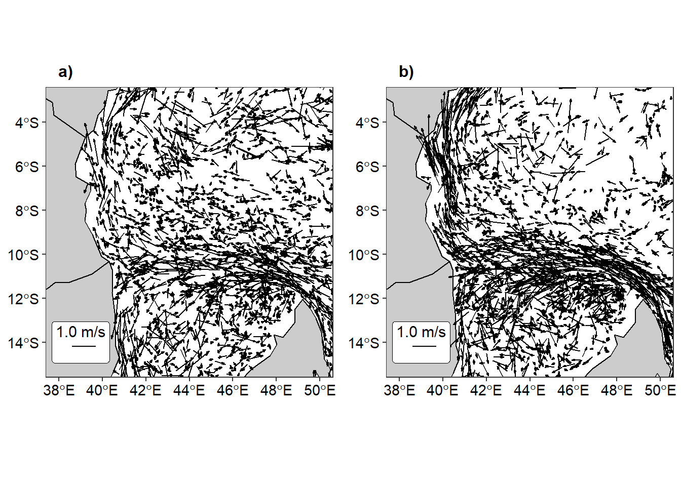
Figure 1: Surface current from drifter observations a)northeast, b)southeast monsoon season

Drifter observation in figure 2 reveals the same picture that the northern branch of the south equatorial current (SEC) in the Indian Ocean passing through the northern extremity of Madagascar Island and continuing westward to the coast of Africa near 11 \({^\circ}\)S. There it splits into the north-flowing East African COastal Current (EACC) and a branch flowing south into the Mozambique Channel. The comparison of surface current in the tropical Indian Ocean suggest that most of the water of the South Equatorial Current goes into the East African Coastal Current than Mozambique Channel (Figure 2).

Like previous studies, drifter reveals clearly the EACC as part of the boundary current system off the East Africa, which flows northward both in northeast (Figure 4) and southeast monsoon season (Figure 3).

Conclusion

Surface current vector (Figure 1) and surface current trajectories (Figure 3 & 4) reveal the previous studies focused on the east african coastal current and south equatorial current. However, the drifter observation show much detailed pathways of the surface current during the southeast and northeast monsoon season.

Cited References