Introduction
Surface Currents are driven by global wind systems that are fueled by energy from the sun1. These currents inturn transfer heat from the tropics to the polar regions, influencing local and global climate2. Ocean currents are an important abiotic factor that significantly influences food webs and reproduction of marine organisms and the marine ecosystems that they inhabit3. Many species with limited mobility depend on this “liquid wind” to bring food and nutrients to them and to distribute larvae and reproductive cells. Even fish and mammals living in the ocean may have their destinations and food supply affected by currents.
Upwelling currents bring cold nutrient-rich waters from the ocean bottom to the surface, supporting many of the most important fisheries and ecosystems in the world4. These currents support the growth of phytoplankton and seaweed which provide the energy base for consumers higher in the food chain, including fish, marine mammals, and humans5.
Despite the importance of ocean current, very little is understood about the circulation pattern in the Pemba Channel. This is contributed by the bottom topographic feature. The channel being the deepest among the the other two channels—Zanzibar and Mafia channel, has hindered placing of oceanographic instruments to continuously measure and monitor the channel. Therefore, in this post, I will try to uncover the seasonal circulation pattern of the channel using the drifter observation from Global Drifter Program.
require(tidyverse)
require(lubridate)
require(leaflet)
require(insol)
require(kableExtra)
require(sf)
require(ggsci)
Processing the data
This post rely on the data processing model proposed by Hadley Wickham in his book R for Data Science6. First step is to import The data. the drifter data were imported them from the local directory into R. This means load the data stored in folder within the machine into the R workspace.
## load the dataset
drifter = read_table2("./drifters.txt", comment = "#",
                      col_names = FALSE)
Once the drifter data was imported into the R environment, it is in the right place to tidy it. Tidying data means storing it in a consistent form that matches the semantics of the dataset with the eay it is stored. Quoting Hadley (2017) stated that the data is tide when each column is a variable, and each row is an observation. Tidy data is an import data processing stage because it organize the data in a consistent structure that help exploration and visualization of data. The tidying of drifter data involved replacing variable names to the ones that make sense and present the variable
# select and renmae the variable
 drifter = drifter%>%select(id = X1, lon = X2, lat = X3, drogue = X4, u = X5, v = X6,
         sst = X7, year = X8, month = X9, day = X10, hour = X11)
Once the drifter data was tidy, it was transformed. Transformation includes combining year, month, day and hour variable into date format that R recognize. Once te date-time variable was create, it was separated into two individual variables—date and time. The drifter dataset comes with dates separated into columns—year, month, day and hour. These four columns were transformed to form date and time presented in table ??
## make date format variable
drifter = drifter%>%
  mutate(date = make_datetime(year = year,
                              month = month,
                              day = day,
                              hour = hour+3,
                              min = 0,sec = 0))


## present the table of time
drifter%>%select(year, month, day, hour, date)%>%separate(date, c("date", "time"), sep = " ")%>%sample_n(10)%>%
  arrange(date)%>%
  kable("html", escape = FALSE, align = "c",
        col.names = c("Year  ", "Month", "Day", "Hour", "Date", "Local Time"),
        caption = "Overview raw drifter date comes as raw and transformed date in R format")%>%
  kable_styling(latex_options = c("striped", "hover"), full_width = TRUE)%>%
  column_spec(1:6, width = "8cm")%>%
  column_spec(5:6, background = "lightseagreen", color = "black", bold = F)%>%
  column_spec(1:4, background = "lightpink", bold = F, color = "black")%>%
  # row_spec(6:10, color = "ivory", background = "#D7261E", bold = T)%>%
  add_header_above(c( "Drifter Date Variables" = 4, "Fomated Date" = 2))%>%
add_header_above(c("Sample Drifter in Pemba" = 6))# span all five columns| Year | Month | Day | Hour | Date | Local Time |
|---|---|---|---|---|---|
| 1998 | 8 | 28 | 0 | 1998-08-28 | 03:00:00 |
| 2002 | 8 | 2 | 0 | 2002-08-02 | 03:00:00 |
| 2003 | 1 | 11 | 18 | 2003-01-11 | 21:00:00 |
| 2003 | 6 | 6 | 18 | 2003-06-06 | 21:00:00 |
| 2003 | 9 | 18 | 18 | 2003-09-18 | 21:00:00 |
| 2005 | 3 | 26 | 12 | 2005-03-26 | 15:00:00 |
| 2005 | 5 | 15 | 0 | 2005-05-15 | 03:00:00 |
| 2007 | 3 | 18 | 0 | 2007-03-18 | 03:00:00 |
| 2011 | 9 | 20 | 6 | 2011-09-20 | 09:00:00 |
| 2013 | 10 | 25 | 6 | 2013-10-25 | 09:00:00 |
The month component was then extracted from the date variable and then used the month information to create monsoon season. The months were grouped into two consipicuous monsoon seasons. The first season was northeast, which includes months from October to March. The second season is the southeast that start in April and span to September.
 pemba =  drifter%>%
  filter(lon >38.8 & lon < 41 & lat >-6,  lat < -4)%>%
  mutate(season = month,
         season = replace(season, season %in% c(10,11,12,1,2,3), "NE"),
         season = replace(season, season %in% c(4,5,6,7,8,9), "SE"))
Once the seasons were determined, a new variable of current velocity was created. Velocity was computed from the meridional (V) and zonal (U) components using the equation (1). The seasonal mean surface current was calculated with equation (2). The sample of the drifter observation is shown in table 2
\[ \begin{equation} Velocity \:(ms^{-1})\:=\: \sqrt{(U^2+V^2)} \tag{1} \end{equation} \]
\[ \begin{equation} \mu \:=\: \sum \: \frac{(n_1 \:+\: n_2 + \:n..... +\: n_\infty)}{N} \tag{2} \end{equation} \]
# compute surface current velocity
pemba = pemba%>%mutate(velocity = sqrt(u^2 + v^2))

pemba%>%separate(date, c("date", "time"), sep = " ")%>%
  select(date, season, lon,lat, u, v, velocity)%>%
  sample_n(12)%>%
  kable("html", align = "c", digits = 2,
        caption = "Overview of the zonal, meridional and surface current velocity",
        col.names = c("Date","Season", "Longitude", "Latitude", "U", "V", "Velocity"))%>%
  kable_styling()%>%
  add_header_above(c("", "Location Information" = 3, "Surface Current" = 3))%>%
  add_header_above(c("" , "Surface Current Information" = 6))%>%
  column_spec(1:6, width = "8cm")%>%
  column_spec(1:2, background = "lightpink", bold = F, color = 1)%>%
  column_spec(3:4, background = "lightgreen", bold = F, color = "black")%>%
column_spec(5:7, background = "lightblue", bold = F, color = "black")| Date | Season | Longitude | Latitude | U | V | Velocity |
|---|---|---|---|---|---|---|
| 2006-10-11 | NE | 39.38 | -4.82 | 0.42 | 0.79 | 0.90 |
| 2002-03-09 | NE | 40.46 | -5.40 | 0.06 | 0.39 | 0.39 |
| 2009-04-21 | SE | 40.38 | -5.62 | -0.25 | 1.15 | 1.18 |
| 2008-12-29 | NE | 40.65 | -5.68 | -0.02 | 0.22 | 0.22 |
| 2009-01-20 | NE | 40.63 | -4.81 | 0.07 | 0.10 | 0.12 |
| 2009-01-18 | NE | 40.57 | -4.85 | 0.04 | 0.14 | 0.14 |
| 2009-10-16 | NE | 40.08 | -4.24 | 0.67 | 0.72 | 0.98 |
| 2015-05-06 | SE | 40.44 | -5.21 | 0.07 | 0.10 | 0.12 |
| 2015-01-21 | NE | 40.49 | -4.87 | -0.15 | 0.05 | 0.16 |
| 2012-04-17 | SE | 40.90 | -5.95 | -0.08 | 0.71 | 0.72 |
| 2015-04-22 | SE | 40.89 | -4.61 | 0.12 | 0.40 | 0.41 |
| 2002-11-20 | NE | 40.05 | -5.29 | 0.15 | 1.16 | 1.17 |
Figure 1 show that the northeast period has higher surface current speed than the northeast monsoon which are randomly distributed between longitude 39 \({^\circ}\)E to 41 \({^\circ}\)E. Thea area in the Pemba Channel between longitude 39.8 \({^\circ}\)E to 40.2 \({^\circ}\)E receive some drifters that moves at a relatively speed above 1.5 ms-1 during the southeast monsoon seasons (Figure 1)
ggplot(data = pemba, aes(x =  lon, y = velocity, col = season))+
  geom_point()+
  stat_ellipse()+
  geom_smooth(se = F, size = 1.2)+
  scale_color_jco(limits = c("SE", "NE"))+
  theme(panel.grid = element_blank(),
        panel.background = element_rect(fill = NA, colour = 1),
        legend.position = c(.92,.85),
        legend.background = element_rect(fill = NA, colour = 1),
        axis.text = element_text(size = 11, colour = "black"),
        axis.title = element_text(size = 12, colour = "black"))+
  scale_x_continuous(breaks = seq(38.5, 41.5,0.5),
                     labels =  scales::unit_format(unit = "E", sep = " ", accuracy = 0.1)) +
  labs(x = "", y = expression(~Surface~Current~Speed~(ms^-1)))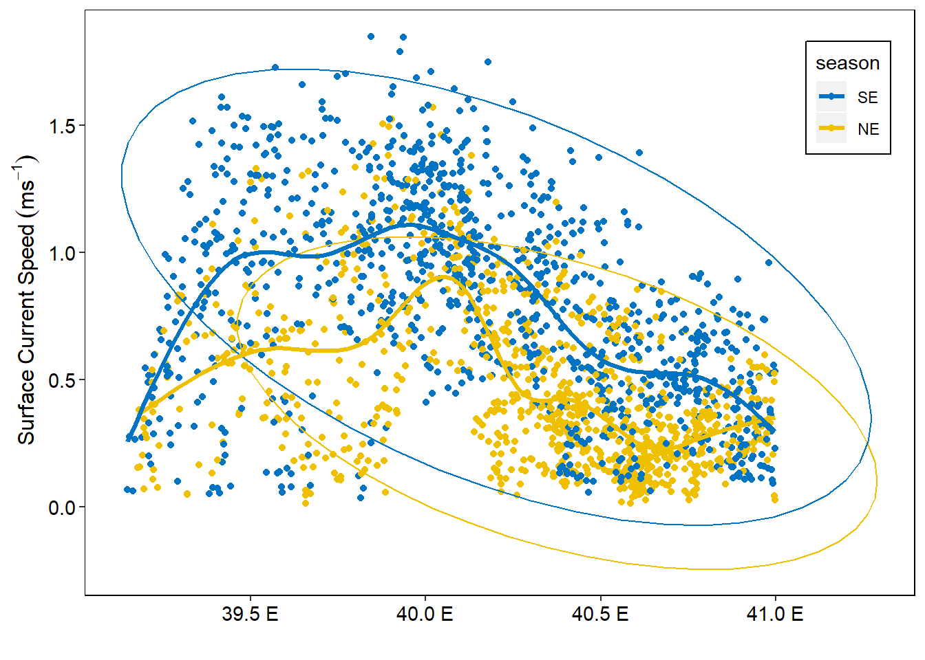
Figure 1: The surface current distribution in the pemba channel
Figure 2 show the seasonal difference of surface current in the Pemba channel. The southeast monsoon has more drifter observation and well distributed surface current (Figure 2b) compared to the northeast monsoon season (Figure 2a)
## current flow

ne.map = ggplot(data = pemba%>%filter(season == "NE"))+
  geom_segment(aes(x = lon, xend = lon+u/8, y = lat, yend = lat+v/8),
               arrow = arrow(angle = 15,length = unit(0.08, "inches"), type = "closed"), col = "black")+
  geom_sf(data = tz.ke, fill = "grey80", col = 1)+
  coord_sf(xlim = c(38.9,40), ylim = c(-5.8,-4.1))+
  scale_x_continuous(breaks = c(39.2, 39.8))+
  scale_y_continuous(breaks = c(-5.5, -4.2))+
  theme_bw()+
  theme(panel.background = element_rect(colour = 1, fill = NA),
        axis.text.x = element_text(colour = 1, size = 11),
        axis.text.y = element_text(colour = 1, size = 11),
        legend.position = "right", panel.grid.major = element_line(colour = NA))+
  geom_label(aes(x = 39.0, y = -5.75, label = "1.0 m/s\n"),
             size = 4, label.padding = unit(0.2, "lines"))+
  geom_segment(aes(x = 38.9, xend = 39.1, y = -5.77, yend = -5.77))+
  labs(x = NULL, y = NULL)

se.map = ggplot(data = pemba%>%filter(season == "SE"))+
  geom_segment(aes(x = lon, xend = lon+u/8, y = lat, yend = lat+v/8),
               arrow = arrow(angle = 15,length = unit(0.08, "inches"), type = "closed"), col = "black")+
  geom_sf(data = tz.ke, fill = "grey80", col = 1)+
  coord_sf(xlim = c(38.9,40), ylim = c(-5.8,-4.1))+
  scale_x_continuous(breaks = c(39.2, 39.8))+
  scale_y_continuous(breaks = c(-5.5, -4.2))+
  theme_bw()+
  theme(panel.background = element_rect(colour = 1, fill = NA),
        axis.text.x = element_text(colour = 1, size = 11),
        axis.text.y = element_text(colour = 1, size = 11),
        legend.position = "right", panel.grid.major = element_line(colour = NA))+
  geom_label(aes(x = 39.0, y = -5.75, label = "1.0 m/s\n"),
             size = 4, label.padding = unit(0.2, "lines"))+
  geom_segment(aes(x = 38.9, xend = 39.1, y = -5.77, yend = -5.77))+
  labs(x = NULL, y = NULL)

cowplot::plot_grid(ne.map, se.map, label_x = 0.2, label_y = 0.98, labels = c("A", "B"))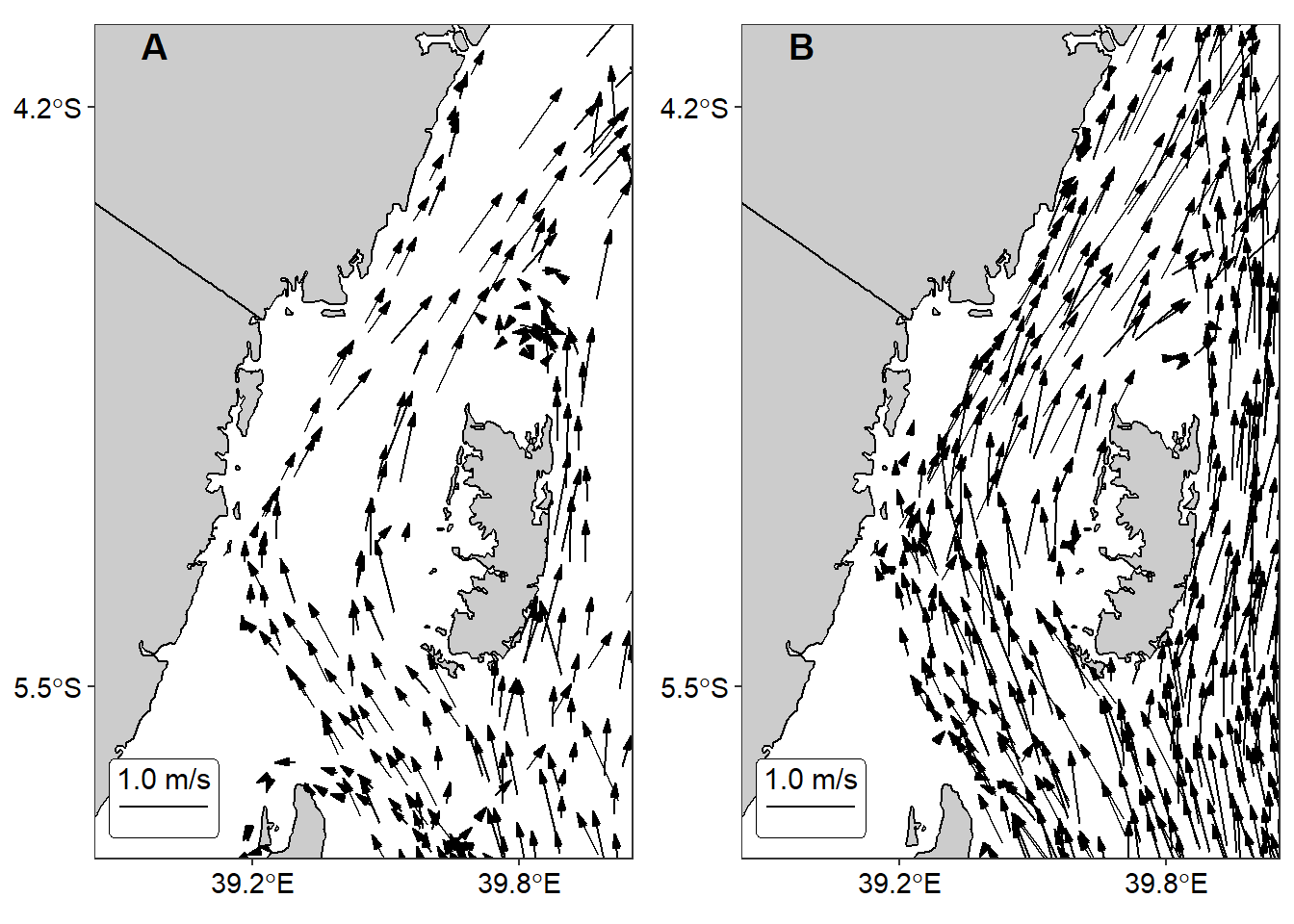
Figure 2: Seasonal variation of surface current vector in the Pemba channel during a) northeast b) and b) southeast monsoon seasons
Cited References
Sverdrup, H. U. (1947). Wind-driven currents in a baroclinic ocean; with application to the equatorial currents of the eastern Pacific. Proceedings of the National Academy of Sciences, 33(11), 318-326.↩
Bryden, H. L., & Hall, M. M. (1980). Heat transport by currents across 25 N latitude in the Atlantic Ocean. Science, 207(4433), 884-886.↩
Treml, E. A., Halpin, P. N., Urban, D. L., & Pratson, L. F. (2008). Modeling population connectivity by ocean currents, a graph-theoretic approach for marine conservation. Landscape Ecology, 23(1), 19-36.↩
Bakun, A. (1990). Global climate change and intensification of coastal ocean upwelling. Science, 247(4939), 198-201.↩
Hutchins, D. A., & Bruland, K. W. (1998). Iron-limited diatom growth and Si: N uptake ratios in a coastal upwelling regime. Nature, 393(6685), 561.↩
Wickham, H., & Grolemund, G. (2016). R for data science: import, tidy, transform, visualize, and model data. " O’Reilly Media, Inc.“.↩