This post introduces to simple analysis of CTD data using oce1 package in R2 environment. CTD stands for conductivity, temperature, and depth, and refers to a package of electronic instruments that measure these properties.A CTD device’s primary function is to detect how the conductivity and temperature of the water column changes relative to depth. Conductivity is a measure of how well a solution conducts electricity. Conductivity is directly related to salinity, which is the concentration of salt and other inorganic compounds in seawater. Salinity is one of the most basic measurements used by ocean scientists. When combined with temperature data, salinity measurements can be used to determine seawater density which is a primary driving force for major ocean currents.
CTDs can provide profiles of chemical and physical parameters through the entire water column. The CTD data used in this post were collected with South African Ship Agulhas II June-July 2018. The ship cruised and made nine casts along the Pemba and Zanzibar channel. This expedition was done under the Second International Indian Ocean Expedition (IIOE–2). The IIOE–2 aim to systematically explore our coastal waters, which are poorly known with prime purpose of discovering and advancing the knowledge.
require(oce)
require(ocedata)
require(sf)
require(leaflet)
require(tidyverse)
Oce package has functions that read the SBE files (.cnv). For example the read.ctd() function read the CTD file directly
stn1 = read.ctd("./ctd18/stn001.cnv")This produce a CTD profile that has both downcast and upcast. Figure 1 for example show the location of the cast on a map and temperature and salinity profiles of raw measurements. You notice that the cast contain bad data for both profiles
par(mfrow = c(1,2))
stn1%>%plot(which = 5)
stn1%>%plot(which = 1)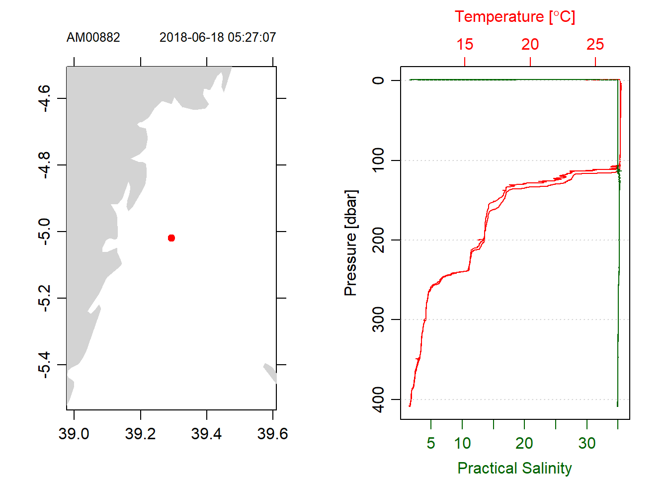
Figure 1: Profile of raw CTD with both downcast and upcast measurements
We can clean the data and remove the bad data, however before we clean the data we must careful choose the casts—whether to select downcast or upcast. oce package has a plotScan() function that help us assess the cast with good data. Figure 2 show the pressure, temperature and salinity measurement against scan number. It is very clear that the first 15000 cast—representing downcast made good measurements and above cast number 15000 we see a jagged lines of poor measurements from the upcast. Note also the spice of temperature and salinity in the downcast scan number.
par(mfrow = c(1,3))

stn1%>%plotScan(which = 1, xtype = "scan", type = "l", main = "Pressure")
stn1%>%plotScan(which = 3, xtype = "scan", type = "l", main = "Temperature")
stn1%>%plotScan(which = 4, xtype = "scan", type = "l", main = "Salinity")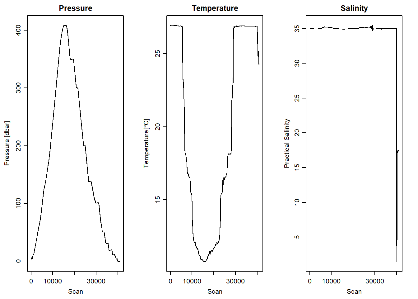
Figure 2: Scan number against pressure, temperature and salinity measurement of raw CTD
Figure 2 reveal the desired downcast measurements and the need to drop the upcast measurement. We can manually trim the upcast using the cut-point of scan number in figure 2, which is 14000. Although the plot for pressure appear pleasing after trimming the upcast manually, we still see some spikes in temperature and salinity (Figure 3)
## Trim upcast scan manually

stn1.clean = stn1%>%
  ctdTrim("range",
          parameters = list(item = "scan",
                            from = 0,
                            to = 14000))
par(mfrow = c(1,3))
stn1.clean%>%plotScan(which = 1, xtype = "scan", type = "l", main = "Pressure")
stn1.clean%>%plotScan(which = 3, xtype = "scan", type = "l", main = "Temperature")
stn1.clean%>%plotScan(which = 4, xtype = "scan", type = "l", main = "Salinity")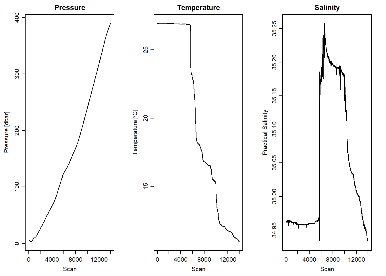
Figure 3: Downcast scan number against pressure, temperature and salinity measurement of manually selected scan number
Kelly & Richards (2007) pointed that selecting values from downcast based on plotted information as the most robust one of trimming CTD data. However, if you work for several cast this method is tedious. It is possible to parse the argument for downcast in the ctdTrim() function to automatically detect the downcast (see figure 4) and the profile of downcast (Figure 5) compared to profiles untrimmed cast (Figure 1).
## purse the downcast argument in ctdTrim to drop the upcast
stn1.d = stn1%>%
  ctdTrim(method = "downcast")

par(mfrow = c(1,3))
stn1.d%>%plotScan(which = 1, xtype = "scan", type = "l", main = "Pressure")
stn1.d%>%plotScan(which = 3, xtype = "scan", type = "l", main = "Temperature")
stn1.d%>%plotScan(which = 4, xtype = "scan", type = "l", main = "Salinity")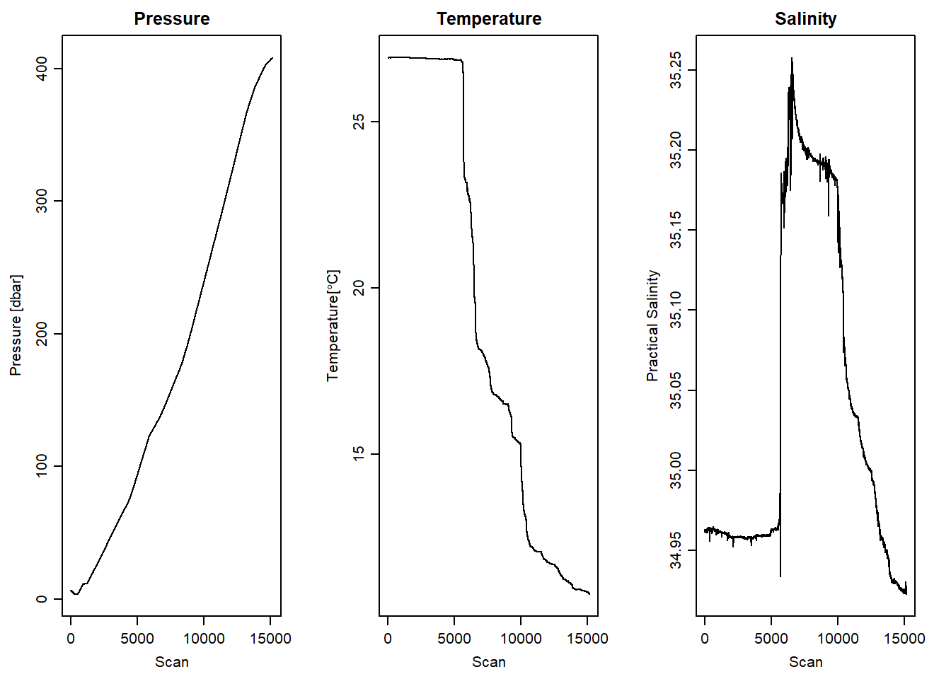
Figure 4: Downcast scan number against pressure, temperature and salinity measurement directy dicted with ctdTrim
par(mfrow = c(1,2))
stn1.d%>%plot(which = 5)
stn1.d%>%plot(which = 1)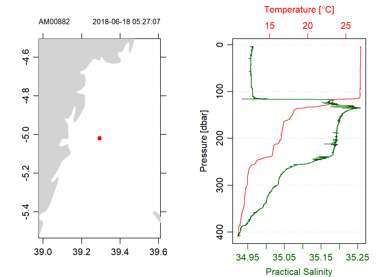
Figure 5: Profiles of trimmed CTD with only downcast measurements
If there are more than one cast that are required for plotting hydrographic section, the casts must be in the same standard pressure. Oce has ctdDecimate() function which handles that issue. It align the CTD data to the standard pressure. For example Figure 6 profiles of temperature and salinity looks cleaner than Figure (fig:fig5) because Figure 6 measurements were aligned in ten meter interval of pressure (chunk below)
## drop the upcast and align in 10 meter interval of pressure
stn1.d = stn1%>%
  ctdTrim(method = "downcast")%>%
  ctdDecimate(p = 10)

par(mfrow = c(1,2))
stn1.d%>%plot(which = 5)
stn1.d%>%plot(which = 1)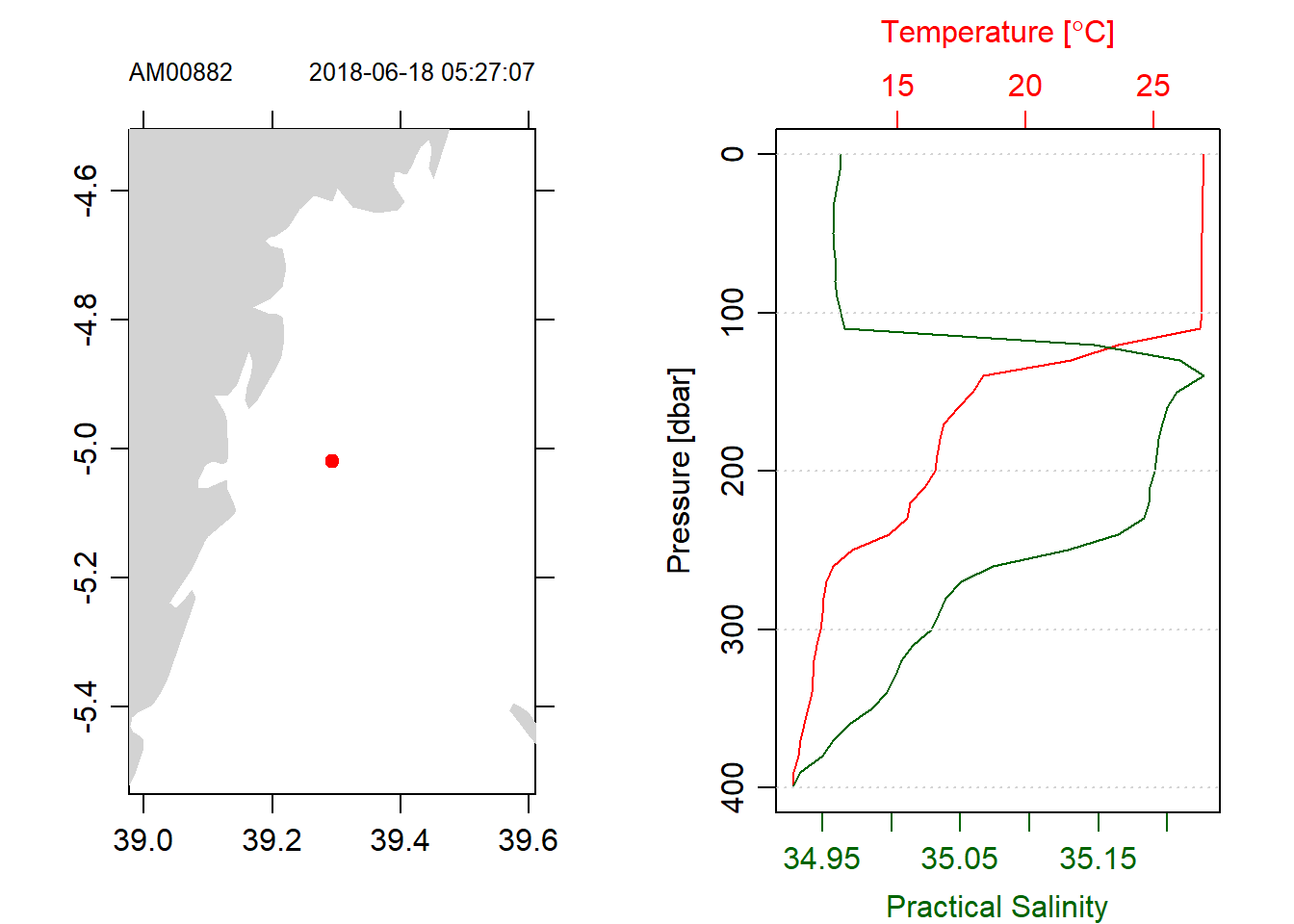
Figure 6: Profiles of trimmed CTD with only downcast measurements aligned in the standard 10 meter interval pressure
So far I have dealing with single CTD cast. Oceanographers often deals with multiple casts,stitched together to form a hydrographic section. Therefore, an iteration is required to process multiple CTD files and R has function to deal with looping routines. For R to iterate, the location of the file and the file path has to be determined.
### Identify the list in the directory
files = dir(path = "./ctd18/", pattern = ".cnv", full.names = TRUE )
The loop through to read the CTD files from the nine stations. However, before we loop, a container to store the files during the looping process is required. I preallocated the file using the list() and then loop the process with a FOR function
## preallocate the container to store the individual
ctd = list()

### Loop the CNV file and create a list of casted CTD
for (i in 1:length(files)){

ctd[[i]]  = read.ctd(files[i])%>%
  ctdTrim(method = "downcast")%>% # select downcast
  ctdDecimate(p = 1) # align to the same standard pressure
}
Because the ctd files for each station are stored as list, a format required for creating section of the nine profiles.
### Make a section of CTD cast from the List
section = ctd%>%as.section()
Figure 7 show the hydrographic section of the nine CTD casts traversed within the Pemba and Zanzibar channel during the southeast monsoon season. The section reveal a similar temperature pattern from surface to 40 meter depth. The range from 26 to 28 ^\(\circ\)C with temperature above 27 lay between latitude 6.5^\(\circ\) and 6.3^ \(\circ\)S (Figure 7).
par(mfrow = c(1,2))
section%>%plot(which = "map", showStations = TRUE, showStart = TRUE)
section%>%plot(which = "temperature", xtype = "latitude", ztype = "image", ylim = c(40,4.5), zlim = c(26,27.8), eos = "gsw")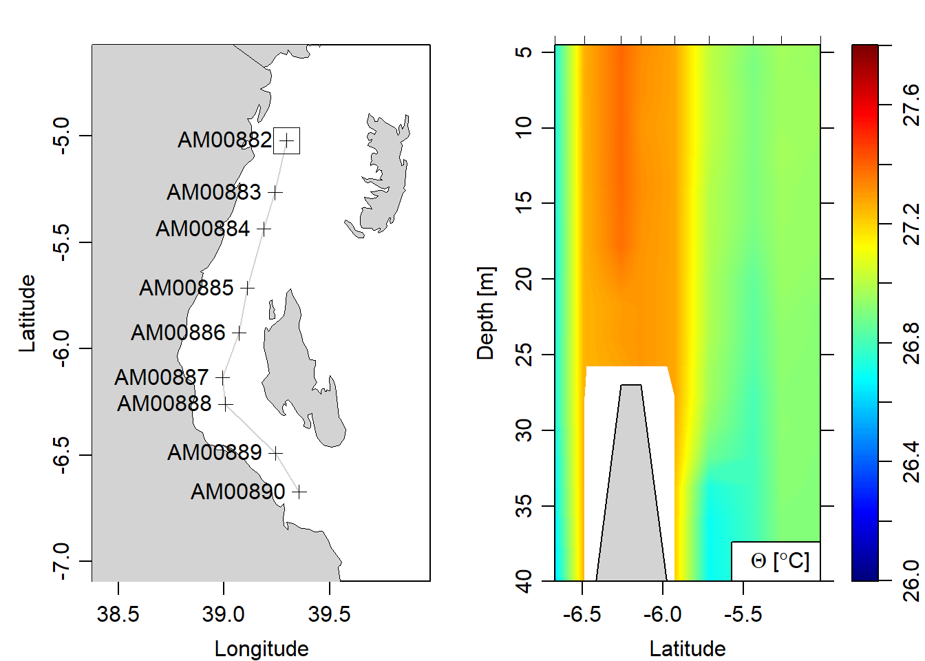
Figure 7: Vertical structure of temperature with the coastal water of 40 meter depth. A map show the location of the CTD stations
Because CTD casts often have different pressure levels at each station, it is recommended to grid them. I will only show how to subset the casts taken in deeper water and then align them to the same pressure levels and plot the sections. The image and contour for temperature (Figure 8), salinity (Figure 9), oxygen (Figure 10), fluorescence (Figure 11) and turbidity (Figure 12).
###subset and grid section
section.gridded = section%>%
  subset(latitude >= -5.5)%>%
  sectionGrid(p = seq(0,500,2))
## plot the gridded section
par(mfrow = c(1,2))
section.gridded%>%
plot(which = "temperature", xtype = "latitude",
ztype = "image", ylim = c(400,4.5),
eos = "gsw")
section.gridded%>%
plot(which = "temperature", xtype = "latitude",
ztype = "contour", ylim = c(400,4.5),
eos = "gsw")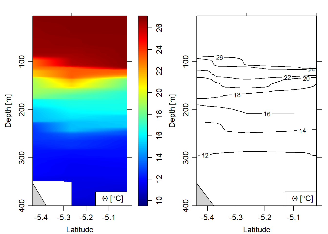
Figure 8: Temperatue section plotted as contour and image
## plot the gridded section

par(mfrow = c(1,2))

section.gridded%>%
  plot(which = "salinity", xtype = "latitude",
       ztype = "image", ylim = c(400,4.5),
       eos = "gsw")

section.gridded%>%
  plot(which = "salinity", xtype = "latitude",
       ztype = "contour", ylim = c(400,4.5),
       eos = "gsw")
Figure 9: Salinity section plotted as contour and image
## plot the gridded section

par(mfrow = c(1,2))

section.gridded%>%
  plot(which = "oxygen", xtype = "latitude",
       ztype = "image", ylim = c(400,4.5),
        eos = "gsw")

section.gridded%>%
  plot(which = "oxygen", xtype = "latitude",
       ztype = "contour", ylim = c(400,4.5),
       eos = "gsw")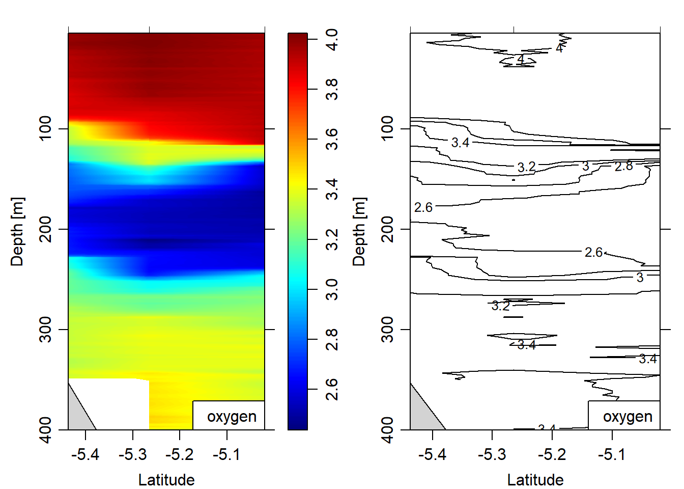
Figure 10: Oxygen section plotted as contour and image
## plot the gridded section

par(mfrow = c(1,2))

section.gridded%>%
  plot(which = "fluorescence", xtype = "latitude",
       ztype = "image", ylim = c(400,4.5),
        eos = "gsw")

section.gridded%>%
  plot(which = "fluorescence", xtype = "latitude",
       ztype = "contour", ylim = c(400,4.5),
       eos = "gsw")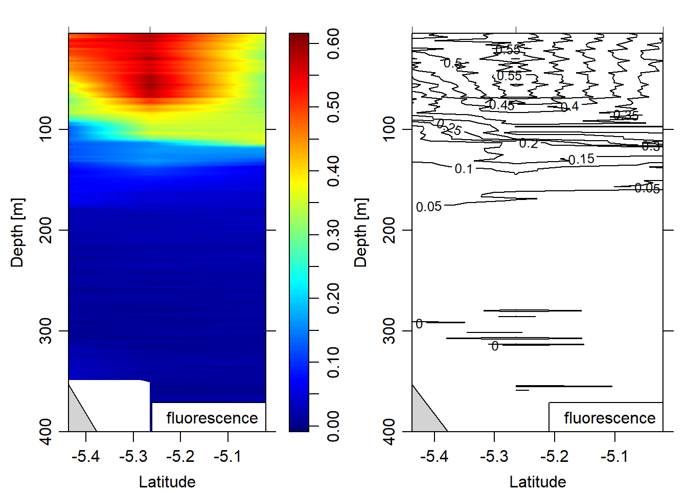
Figure 11: Fluorescence section plotted as contour and image
## plot the gridded section

par(mfrow = c(1,2))

section.gridded%>%
  plot(which = "turbidity2", xtype = "latitude",
       ztype = "image", ylim = c(400,4.5),
        eos = "gsw")

section.gridded%>%
  plot(which = "turbidity2", xtype = "latitude",
       ztype = "contour", ylim = c(400,4.5),
       eos = "gsw")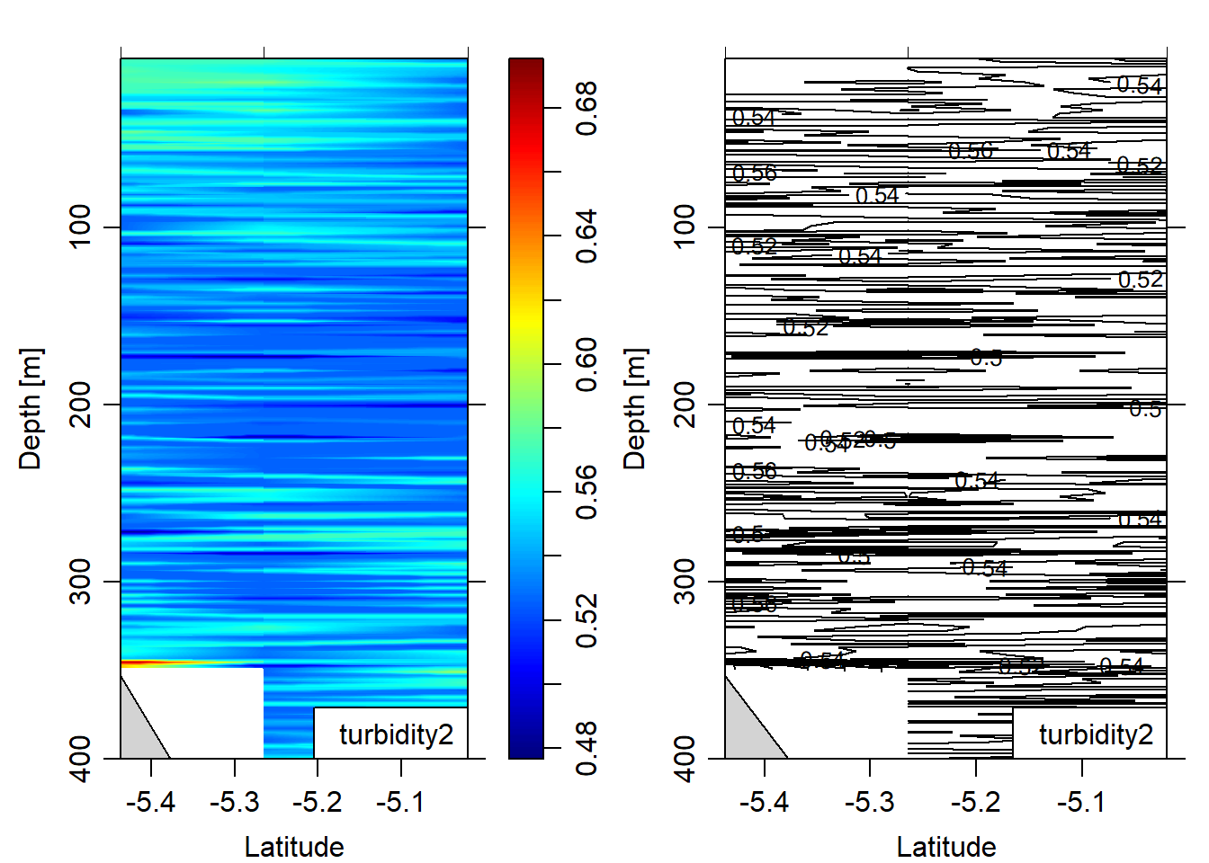
Figure 12: turbidity section plotted as contour and image
Make a data frame of CTD cast from the List
We have seen the oce package make it eay to read, summarize and visualize CTD data. So far we dealt with oce package processing and plotting, which use base graphic package. The next post will deal with tranforming oce dataset format into a tibble—a modern data frame. A tibble allows to tidy3, manipulate4 CTD data and visualize5 profiles and section easily with tidyverse6.
Cited Literature
Kelley, D., & Richards, C. (2017). oce: Analysis of Oceanographic Data. R package version 0.9-22.↩
Team, R. C. (2015). R: A language and environment for statistical computing.↩
Wickham, H. (2016). tidyr: Easily Tidy Data with spread () and gather () Functions. Version 0.6. 0.↩
Wickham, H., Francois, R., Henry, L., & Müller, K. (2015). dplyr: A grammar of data manipulation. R package version 0.4, 3.↩
Wickham, H. (2016). ggplot2: elegant graphics for data analysis. Springer.↩
Wickham, H. (2017). Tidyverse: Easily install and load’tidyverse’packages. R package version, 1(1).↩