Introduction
In this post, I am going to illustrate routines of how to validate sea surface temperatures from Moderate Resolution Imaging Spectroradiometer (MODIS) with drifters’ sea surface temperature. Drifters measurements serve as in-situ data against MODIS data. The purpose is to assess closeneness (accuracy) of satellite and in-situ SST. I will check the accuracy of acquired (satellite) and measured (drifter) SST, visualize their relationship and test the significance of the relationship.
Needed Packages
Several packages are needed for this routine (this assumes are installed already in the machine).
require(tidyverse)
require(insol)
require(lubridate)
require(sf)
require(oce)
require(ocedata)
require(leaflet)
require(xtractomatic)
require(rerddapXtracto)
Drifter data
The drifter data downloaded from Global Drifter Program as tab delimited was imported into R workspace using the read_table2() function of readr1 package. Once the file was in the workspace, the column variables were assigned proper names.
## read drifter dataset
drifters = read_table2("./drifters.txt",
                       col_names = FALSE, comment = "#")

## rename the variables to their respective variable names
drifters = drifters%>%
  select(id = 1, lon = 2, lat = 3,
         drogue = 4,  u = 5, v = 6, sst = 7,
         year = 8, month =9, day = 10, hour = 11)
Transform date
The dataset comes with four columns that present date—year, month, day, and hour. These variables were converted to date in R using the JDymd() function of insol2 package. The date transformation involved two steps–converting to year, month, day variable into julian day and then convert the julian day to gregorian calendar. Once the date aligned with R format, the year, month, day and hour variables were dropped from the drifter dataset. The data in table 1 show the date, identification number longitude, latitude and sea surface temperature of fifteen randomly selected drifters.
| Date | ID | Longitude | Latitude | Zonal (U) | Meridional (V) | SST |
|---|---|---|---|---|---|---|
| 2008-10-19 | 53417 | 42.72 | -10.46 | -0.34 | 0.03 | 27.03 |
| 2015-11-22 | 132486 | 50.87 | -10.67 | -0.66 | 0.12 | 28.27 |
| 2000-06-06 | 18871 | 47.97 | -7.51 | 0.18 | -0.33 | 26.30 |
| 2014-02-25 | 109550 | 41.53 | -4.51 | 0.52 | -0.62 | NaN |
| 2006-08-17 | 57899 | 39.81 | -8.32 | 0.30 | 0.90 | NaN |
| 1999-03-25 | 9706574 | 46.71 | -6.62 | 0.50 | 0.20 | 30.70 |
| 2008-10-30 | 71201 | 48.16 | -11.95 | -0.04 | -0.07 | 26.78 |
| 2016-05-05 | 101833 | 49.16 | -1.02 | 0.26 | 0.50 | NaN |
| 2013-06-24 | 109404 | 40.75 | -10.48 | -0.48 | 0.72 | 25.31 |
| 2009-09-11 | 63875 | 42.18 | -15.79 | 0.88 | -0.62 | 25.86 |
| 2008-12-06 | 70851 | 47.02 | -11.81 | 0.25 | -0.57 | 28.14 |
| 1996-11-26 | 9421930 | 40.03 | -7.12 | -0.24 | 0.90 | NaN |
| 2008-12-03 | 70859 | 48.61 | -11.95 | 0.33 | 0.26 | 28.18 |
| 2017-08-22 | 63943940 | 42.98 | -1.69 | -0.05 | 0.09 | 26.41 |
| 2001-08-27 | 25006 | 45.44 | -9.41 | -0.79 | -0.43 | 24.33 |
Drifter selection
There are 94413 observations from 466 unique drifters. However, drifter 70973 was selected for validation. This drifter begun its way at latitude -14.213 \(^{\circ}\)S and longitude 51.995 \(^{\circ}\)E on 2010-11-02 and finished near Nungwi at latitude -5.722 \(^{\circ}\)S and longitude 39.32 \(^{\circ}\)E on 2011-01-22. During its journey, which took 81 days covering a distance of 2561.29 kilometers, it made 326 observations (Figure 1).
Figure 1: Sample locations of drifter with Id 70973 crossed within the tropical indian ocean
Using the drifter geographical position, a simple feature was created that was used to create trajectory—a pathway along which drifter made several observation on its route (Figure 2)
## create a simple feature from tibble
drifter.sf = drifters%>%
  st_as_sf(coords = c("lon", "lat"))%>%
  st_set_crs(4326)

## make a trajectory form the simple feature points
drifter.traj = drifter.sf%>%
  group_by(id)%>%
  summarise(do_union = FALSE)%>%
  st_cast("LINESTRING")

## make a map of trajectory
leaflet(data = drifter.traj%>%filter(id == 70973))%>%
  addTiles()%>%
  addPolylines(color = "red", stroke = T, weight = 2.5)
Figure 2: The Trajectory of Drifter with Id 70973, which crossed the tropical indian ocean for a period of one year
Modis Data
The selected drifter dataset contains three variables—date, longitude and latitude of the drifter observation. These observations serves as trackline and was used to extract sea surface temperature from MODIS satellite. xtracto() function from xtractomatic3 package was used for extraction. Let’s explore the metadata of the ERDAPP servers that deals with sst
We observed that the MODIS sst dataset span from 2003-01-05 to 2018-08-25 covering all the global oceans at spatial resolution of 4.0866. The function xtracto() was used to extract sea surface temperature along the trackline of selected drifter with Id 70973.
## extract sst along the trackline of drifter
sst_modis = xtracto(dtype = "mhsstd8day",
              xpos = drifter.70973$lon,
              ypos = drifter.70973$lat,
              tpos = drifter.70973$date, ,
              xlen = 0.2,
              ylen = 0.2)
Stitching Drifter and MODIS dataset
Once the data was extracted from MODIS and loaded in the workspace, it was cleaned by removing variables not needed and then bind it with the drifter dataset using the bind_cols() function from dplyr4 package.
sst.modis.clean =sst_modis%>%
  select(satellite.date = 4,
         satellite.sst.mean = 1,
         satellite.sst.median = 10 )

## bind the drifter data and extracted modis data
drifter.modis = drifter.70973%>%
  select(drifter.date = date, lon,lat, drifter.sst = sst)%>%
  bind_cols(sst.modis.clean)%>%select(1,5,2,3, 4, 6,7)%>%
  mutate(satellite.date = as.Date(satellite.date))
The table 2 highlight information of of drifter and satellite sea surface temperature that were marked at the same geographical location. There are mismatch of Some drifter observations to the satellite data. This is because the modis data takes three days to cover the entire world and the day that satellite passed the region might misses some drifter observation.
## clean the data set and remove variables not wanted

knitr::kable(drifter.modis%>%dplyr::sample_n(20),
             align = "c", digits = 2,
             col.names = c("Drifter Date","Modis Date","Longitude","Latitude",
                           "Drifter SST","Satellite SST Mean",
                           " Satellite SST Median") ,
caption = "Overview of merged drifter and satellite dataset")| Drifter Date | Modis Date | Longitude | Latitude | Drifter SST | Satellite SST Mean | Satellite SST Median |
|---|---|---|---|---|---|---|
| 2010-11-04 | 2010-11-05 | 51.55 | -14.39 | 26.39 | 26.43 | 26.45 |
| 2010-11-24 | 2010-11-21 | 50.72 | -15.49 | 26.91 | 26.58 | 26.60 |
| 2010-12-15 | 2010-12-15 | 50.83 | -13.36 | 28.09 | 27.27 | 27.27 |
| 2010-12-23 | 2010-12-23 | 47.97 | -10.91 | 28.52 | 28.37 | 28.35 |
| 2010-11-19 | 2010-11-21 | 50.65 | -15.62 | 26.53 | 26.34 | 26.39 |
| 2010-11-17 | 2010-11-13 | 50.60 | -15.26 | 26.44 | 26.21 | 26.22 |
| 2011-01-08 | 2011-01-05 | 40.64 | -9.39 | 29.40 | 29.53 | 29.48 |
| 2011-01-06 | 2011-01-05 | 40.73 | -9.44 | 29.14 | 29.56 | 29.44 |
| 2010-11-10 | 2010-11-13 | 50.55 | -14.55 | 26.30 | 26.07 | 26.06 |
| 2010-11-18 | 2010-11-21 | 50.66 | -15.52 | 26.85 | 26.50 | 26.54 |
| 2010-11-16 | 2010-11-13 | 50.43 | -15.03 | 26.26 | 26.29 | 26.25 |
| 2010-11-22 | 2010-11-21 | 50.60 | -15.55 | 27.02 | 26.28 | 26.26 |
| 2010-12-08 | 2010-12-07 | 51.34 | -14.74 | 27.63 | 27.32 | 27.31 |
| 2010-11-30 | 2010-11-29 | 51.03 | -15.37 | 27.47 | 26.99 | 27.01 |
| 2010-11-21 | 2010-11-21 | 50.52 | -15.47 | 27.09 | 26.36 | 26.38 |
| 2010-12-01 | 2010-11-29 | 51.08 | -15.27 | 27.64 | 26.94 | 26.98 |
| 2010-11-12 | 2010-11-13 | 50.33 | -14.64 | 26.30 | 26.20 | 26.10 |
| 2011-01-14 | 2011-01-13 | 40.10 | -8.41 | 29.52 | 29.21 | 29.22 |
| 2010-12-18 | 2010-12-15 | 50.10 | -12.37 | 28.21 | 27.40 | 27.44 |
| 2011-01-02 | 2011-01-05 | 41.44 | -9.66 | 29.31 | 31.30 | 31.35 |
Validation
rmse = pracma::rmserr(drifter.modis$drifter.sst,
                      drifter.modis$satellite.sst.mean,
                      summary = FALSE)

estimator = c("Mean Absolute", "Mean Squared",
              "Root Mean Square","Mean Absolute Percentage",
              "Normalized Mean Squared","Relative Standard Deviation")

rmse.t = rmse%>%
  as.data.frame()%>%
  t()%>%
  as.data.frame()%>%
  rename("Error" = V1)%>%
  data.frame(estimator)%>%
  as.tibble()%>%
  select(2,1)%>%
  arrange(Error)
To assess the accuracy of MODIS sea surface temperature, I tested MODIS data against drifter observations using six different algorithms (Table 3). The Mean Absolute Percentage algorithm had the highest accuracy of 0.014906\(^{\circ}\) Celcius and the Root Mean Square achieved the lowest accuracy of 0.5587292\(^{\circ}\) Celsius. In general, the sea surface temperature from modis showed a mean accuracy of 0.261438\(^{\circ}\) Celsius.
knitr::kable(rmse.t,
             digits = 2,
             align = "l",
             col.names = c("Estimator", "Value (Degree Celsius)"),
caption = "Error estimates of surface current with various tools")| Estimator | Value (Degree Celsius) |
|---|---|
| Mean Absolute Percentage | 0.01 |
| Relative Standard Deviation | 0.02 |
| Normalized Mean Squared | 0.24 |
| Mean Squared | 0.31 |
| Mean Absolute | 0.42 |
| Root Mean Square | 0.56 |
## computing the correlation coefficient
pear = cor.test(drifter.modis$drifter.sst,
                drifter.modis$satellite.sst.mean)
The accuracy of the sea surface temperature is also supported by Figure 3, which show the positive association of sea surface temperature between in-situ drifter observations and MODIS satellite data (R2 = 0.92). This association was significant ( t_(1,324)_ = t < 41.5847664 , p = 5.951450210^{-132})
ggplot(data = drifter.modis,
       aes(x = drifter.sst, y = satellite.sst.mean))+
  geom_point()+
  geom_smooth(fill = "green", col = "red")+
  theme(panel.background = element_rect(colour = 1),
        axis.text = element_text(colour = 1, size = 12),
        axis.title = element_text(colour = 1, size = 14))+
 geom_text(aes(x = 29, y = 26,
               label = paste("RSq = ", 0.92)), size = 4)+
  scale_x_continuous(breaks = seq(25.5,31, .5))+
  scale_y_continuous(breaks = seq(26,31, 1.5))+
    labs(y=expression(~Modis~Sensor~SST~(~degree~C)),
         x=expression(~Drifter~Temperature~(~degree~C)))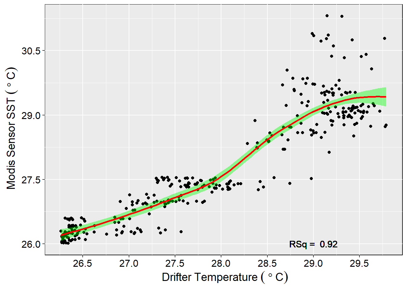
Figure 3: Association of sea surface temperature from in-situ drifter observation and MODIS
Conclusion
Comparing MODIS satellite and drifter sea surface temperature showed a close match with an accuracy of 0.261438\(^{\circ}\) Celsius and a strong and significant positive correlation (R2 = 0.92). The closeness of drifter and MODIS sea surface temperature allows scientists in the region to use MODIS satellite data to tackle marine and coastal issues in the region.
References
Wickham, H., Hester, J., & Francois, R. (2016). Readr: read tabular data. URL https://github. com/hadley/readr. R package version 0.1, 1, 361.↩
Corripio, J. G. (2014). Insol: solar radiation. R package version, 1(1), 2014.↩
Mendelssohn, R. (2017). xtractomatic: accessing environmental data from ERD’s ERDDAP server. R package version, 3(2).↩
Wickham, H., Francois, R., Henry, L., & Müller, K. (2015). dplyr: A grammar of data manipulation. R package version 0.4, 3.↩