During the last couple of decades, Matlab has been the most commonly-used scripting language in physical oceanography (Bengtsson 2018), and it has a large user base in many other fields. However, Python has been gaining ground, often being adopted by former Matlab users as well as by newcomers. Here is a little background to help you understand this shift, and why we advocate using Python from the start.
Python was designed by a computer scientist as a general–purpose scripting language for easy adoption and widespread use. People tried it and liked it, and the result is that it is widely used throughout the software world, for all sorts of tasks, large and small. There is a vast array of Python packages that are freely available to do all sorts of things—including the sorts of things that oceanographers and other scientists do; but these packages are not neatly bound up in a single product, and the documentation for the language itself and for the packages is similarly scattered and of varying quality.
Why I think we should use open source software package like Python instead of proprietary programming language? Like R, Python is fundamentally a better computer language in many ways and free open software with large community support.
- It is suitable for a wider variety of tasks.
- It scales better from the shortest of scripts to large software projects.
- It facilitates writing clearer and more concise code.
- With associated tools, it makes for easier access to existing high-performance codes in compiled languages, and for using smaller pieces of compiled code to speed up critical sections.
- Because Python is Free and Open Source Software (FOSS), you can install it on any machine without having to deal with a license manager.
- For the same reason, Python code that is part of a research project can be run by anyone, anywhere, to verify or extend the results.
- Most Python packages you are likely to want to use are developed in an open environment. The scientific Python ecosystem is dynamic and friendly.
The usefulness of Python for data science stems primarily from the large and active ecosystem of third-party packages: NumPy for manipulation of homogeneous array based data, Pandas for manipulation of heterogeneous and labeled data, SciPy for common scientific computing tasks, Matplotlib for publication-quality visualizations, and Scikit-Learn for machine learning, and related tools–to effectively store, manipulate, and gain insight from data.
Let’s us configure our session so that we can make full access of Python language in R Studio. We do that by loading a reticulate package first before we configure as the chunk below highlight;
require(reticulate)
use_python("c:/Python/Anaconda3/")
Once we have configured the Python environment in R, we must also load some module from R into Rstudio. This will make the functions in these module available for our processing and plotting. We use the convention naming of Python package as seen in the chunk below.
Note that loading Python modules in R session must be done inside the Python chunk. Otherwise you get an error message or a chunk fail to iterate the process
import netCDF4 as nc
import numpy as np
import pandas as pd
import seaborn as sns
# from mpl_toolkits.basemap import Basemap
Data
We will use temperature data for this post. This dataset can be obtained from the Group of High Resolution Sea Surface Temperature (GHRSST) from this. We then use nc.Dataset function from netCDF4 module to read the NetCDF file
sst = nc.Dataset("e:/MatlabWorking/GHRSST/20150101.nc")We then use a . function to access the variables in the dataset
sst.variablesOrderedDict([('lat', <class 'netCDF4._netCDF4.Variable'>
float32 lat(lat)
long_name: latitude
standard_name: latitude
axis: Y
units: degrees_north
comment: uniform grid from -89.875 to 89.875 by 0.25
unlimited dimensions:
current shape = (720,)
filling on, default _FillValue of 9.969209968386869e+36 used
), ('lon', <class 'netCDF4._netCDF4.Variable'>
float32 lon(lon)
long_name: longitude
standard_name: longitude
axis: X
units: degrees_east
comment: uniform grid from -179.875 to 179.875 by 0.25
unlimited dimensions:
current shape = (1440,)
filling on, default _FillValue of 9.969209968386869e+36 used
), ('time', <class 'netCDF4._netCDF4.Variable'>
int32 time(time)
long_name: reference time of sst field
standard_name: time
axis: T
units: seconds since 1981-01-01 00:00:00
unlimited dimensions:
current shape = (1,)
filling on, default _FillValue of -2147483647 used
), ('analysed_sst', <class 'netCDF4._netCDF4.Variable'>
int16 analysed_sst(time, lat, lon)
long_name: analysed sea surface temperature
standard_name: sea_surface_temperature
type: foundation
units: kelvin
_FillValue: -32768
add_offset: 273.15
scale_factor: 0.01
valid_min: -300
valid_max: 4500
unlimited dimensions:
current shape = (1, 720, 1440)
filling on), ('analysis_error', <class 'netCDF4._netCDF4.Variable'>
int16 analysis_error(time, lat, lon)
long_name: estimated error standard deviation of analysed_sst
units: kelvin
_FillValue: -32768
add_offset: 0.0
scale_factor: 0.01
valid_min: 0
valid_max: 127
unlimited dimensions:
current shape = (1, 720, 1440)
filling on), ('mask', <class 'netCDF4._netCDF4.Variable'>
int8 mask(time, lat, lon)
long_name: sea/land field composite mask
_FillValue: -128
flag_values: 1
flag_meanings: sea land lake ice
comment: b0:1=grid cell is open sea water b1:1=land is present in this grid cell b2:1=lake surface is present in this grid cell b3:1=sea ice is present in this grid cell b4-b7:reserve for future grid mask data
unlimited dimensions:
current shape = (1, 720, 1440)
filling on), ('sea_ice_fraction', <class 'netCDF4._netCDF4.Variable'>
int8 sea_ice_fraction(time, lat, lon)
long_name: sea ice area fraction
standard_name: sea ice area fraction
units: percent
_FillValue: -128
add_offset: 0.0
scale_factor: 0.01
valid_min: 0
valid_max: 100
unlimited dimensions:
current shape = (1, 720, 1440)
filling on)])Extracting the variables
The need to separate variable should be done after you have explored how the data is structured and how the variableas are organized. for drawing maps, we need three variables, longitude,latitude and temperature. These has to be extracted from the netcdf file. We notice that the dataset is an array with time, lon, lat and analysed_sst variables. We can simply extract the variables as the chunk below highlight.
time = sst.variables['time']
lon = sst.variables['lon']
lat = sst.variables['lat']
data = sst.variables['analysed_sst']
Once we have extracted the variables from the dataset, we can check the dimension of the
data.dimensions('time', 'lat', 'lon')Visualization with Matplotlib
Matplotlib is a multiplatform data visualization library built on NumPy arrays, and designed to work with the broader SciPy stack. One of Matplotlib’s most important features is its ability to play well with many operating systems and graphics backends. Matplotlib supports dozens of backends and output types, which means you can count on it to work regardless of which operating system you are using or which output format you wish.
Before we dive into the details of creating visualizations with Matplotlib, there are a few useful things you should know about using the package. Just as we use the np shorthand for NumPy and the pd shorthand for Pandas, we will use some standard shorthands for Matplotlib imports:
import matplotlib.pyplot as pltThe plt interface is what we will use to plot sea surface temperatue in this post. Because we are using Matplotlib from within a script, the functionplt.show() is our friend. plt.show() starts an event loop, looks for all currently active figure objects, and display your figure or figures. For all Matplotlib plots, we start by creating a figure and an axes. In their simplest form, a figure and axes can be created as follows
fig, axes = plt.subplots(nrows=1, ncols=1)
plt.imshow(data[0,:,:]-273,)
plt.colorbar()
<matplotlib.colorbar.Colorbar object at 0x0000000034BBE708>plt.show()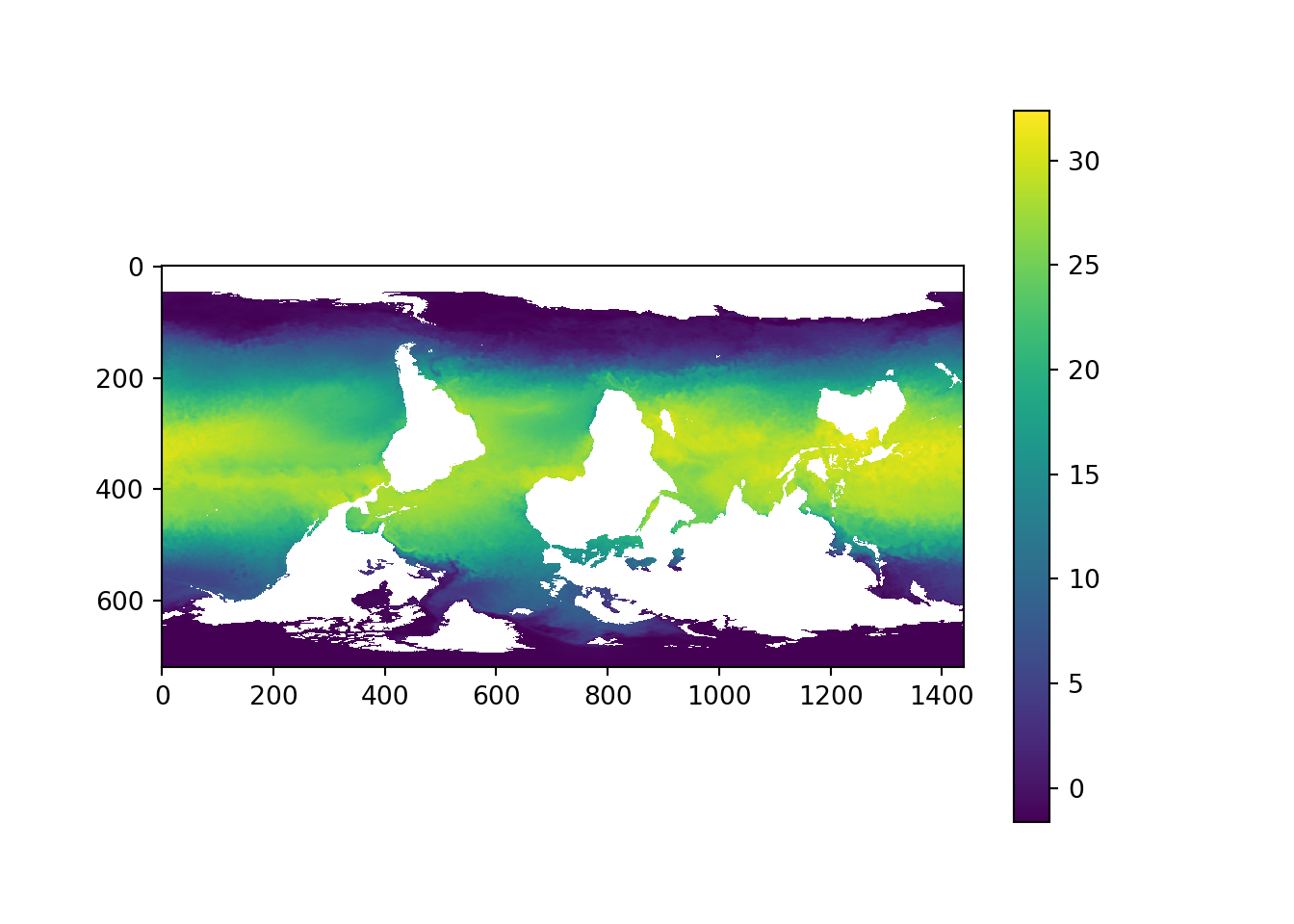
Figure 1: Global Sea surface temperature
The plt.show() command does a lot under the hood, as it must interact with your system’s interactive graphical backend.
From figure 1, we notice the figure is flipped upside down. we need to correct the data and map it in the correct orientation. we use np.flipud function from numpy module for correcting the orientation. we can correct the array using a flipud function from NumPy module.
datar = np.flipud(data[0,:,:]-273)

fig, axes = plt.subplots(nrows=1, ncols=1)
plt.imshow(datar, cmap = "jet")
plt.colorbar()
<matplotlib.colorbar.Colorbar object at 0x0000000034C45308>plt.clim(5,30)
plt.show()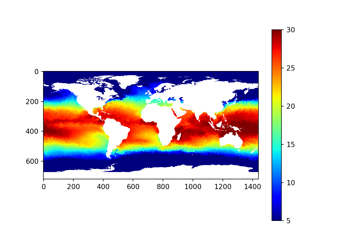
Figure 2: Corrected sea surface temperature
Cited Material
Bengtsson, Henrik. 2018. R.matlab: Read and Write Mat Files and Call Matlab from Within R. https://CRAN.R-project.org/package=R.matlab.