The the National Examinations Council of Tanzania publishes Primary and Secondary Education Examination Results. But the National Library Services archieve this results. While a fantastic resource for history primary and secondary school results, these records are painful to analyze using software because of the grades results is organized is untidy and in messy.
You need to work on this column of the result to have a clean and right format dataset for exploration and modelling. The tidyverse ecocystem has two excellent packages for manipulating files that are not amenable to analysis because of inconsistencies and structure: tidyr provides many tools for cleaning up messy data, dplyr provides many tools for restructuring data.
The tables are in HTML tables—a standard way to display tabular information online. But tables on the web are primarily designed for displaying and consuming data, not for analytical purposes. To make working with HTML tables easier and less time-consuming, Christian Rubba (2016) developed a htmltab package for the R system that tries to alleviate these problems directly in the parsing stage when the structural information is still available.
Load Packages
This post uses R packages, which are collections of R code that help users code more efficiently. We load these packages with the function require(). The specific packages we’ll use here include tidyverse for data manipulation and visualization (Wickham 2017) and htmltab to import HTML tables into data frame (Rubba 2016) and readxl for export of the structured dataset into Excel (Wickham and Bryan 2018). If you have not installed any of these packages before, you will need to do so before loading them (if you run the code below prior to installing the packages, you should see a message indicating that the package is not available). If you have installed these before, then you can skip this step.
You can install these package, as follows:
packs = c("tidyverse", "htmltab)

install.packages(packs)
Once you have installed the package, you can simply them into your session using a require() function. Please note that you only need to install the package once, and when is already installed, the next time you want to use it you simply load it into the session.
require(tidyverse)
require(htmltab)
The 2019 Secondary Education Results
I will use a 2019 Form IV results to demostrate the idea. The results are hosted at this link. Is a HTML table and we can only read this using the right function in R. For this post I will use the htmltab function from htmltab package (Rubba 2016). At a minimum, htmltab() needs to be fed the HTML document as well as an information where to find the table in the page. After a bit of testing out , I found that it is the 3rd table in the page, so I pass 9 to the which argument:
index = htmltab::htmltab(doc = "https://maktaba.tetea.org/exam-results/CSEE2019/csee.htm", which = 3)We can print the dataset to have a glimpse of the ten rows. We notice that the file structure is similar to the table format in the html document. It contains three columns. But the function used the first row observation as the column names. We need to structure the data and ensure Ilboru is one of the observation of the dataset and not the variable name. We give the data its contents
index %>%
  # head() %>%
  as_tibble()
Create School Index
We need to create a data frame that has three columns for school index, school name and the year of exam results. With that dataset will be able to pull results of each school. First we need to change the variable name in the index dataset into rows, there is no straight function to do that particular task, I created a simple function to that for me. This function will return the data frame with columns as observation, which is actually what is suppose to be.
var2row = function(x){

  require(tidyverse)

  data = x %>%
     names() %>%
     t() %>%
     as_tibble() %>%
     rename(column1 = 1, column2 = 2, column3 = 3)

  return(data)
}
Once we have created the function, we can use to create the firs row of observation in the dataset from the index dataset. We simply return the observation in its place
firs.row = index %>%
  var2row()

firs.row
We can now stitch the first row data we simply created above with the observation in the index dataset. We do that using abind_rows function from dplyr package (Wickham et al. 2018). We need to change the column names for the index dataset to match those in the firs.row dataset before we bind them.
## rename
index = index %>%
     rename(column1 = 1, column2 = 2, column3 = 3)

## stitch them together
index = firs.row %>%
  bind_rows(index)
The index structure is in the format widely known as wide format, but we need to transform it to long format. I use a pivot_longer function from dplyr package to transform the dataset (Wickham et al. 2018).
`
index = index %>%
     pivot_longer(cols = 1:3, names_to = "column", values_to = "school")

index
The pivot_longer function changes the shape of the dataset from three columns to two. It moves the variable names to a new columnand all school to a new school column, which contains the index and name of each school as observations.
We also need to separate the index and school name into separate columns. We can do that using the separate function from tidyr package (Wickham and Henry 2018). Careful looking on the index is the mixture of letter and number forming a five number characters. We can use this as a criterion to separate the school into index and name and add a new column using a mutate function form dplyr package (Wickham et al. 2018)
schools.index =  index %>%
     select(-column) %>%
     separate(col = school, into = c("index", "name"), sep = 5) %>%
     mutate(index = tolower(index)) %>% mutate(year = 2019)

schools.index
Dowload the schoool result
In section we only need to prepare the dataset in a proper format. This index is then used to download the results for each school. The code below will download results for each school results in 2019. Because there are 5000 school results, its tedious to do manually, instead I use the power programming to iterate the process. It use for loop to iterate. The loop create a tag which correspond the HTML url for each school. Once the the tag is created, is fed into the htmltab function, which download the HTML table as data frame. Then the name, index and year columns are added for each school. In summary, the iteration prepare a tag file for each school and download and reorganize the data in tabular form for each school. Once the result for a school is download and organized is stored in the list file that is created as container .
necta2019 = list() ## preoccupied file to store list file for each shool results

for (i in 1:nrow(schools.index)){

  ## create a tag for each school
  tag = paste0("https://maktaba.tetea.org/exam-results/CSEE2019/",schools.index$index[i],".htm")

  ## read a tag and mutate variable for each school
  necta2019[[i]] = htmltab::htmltab(doc = tag, which = 3)  %>%
      mutate(index = schools.index$index[i],
             school = schools.index$name[i],
             year = schools.index$year[i]) %>%
        as_tibble()

}
Create table from a list
The function bind_rows was used to stitch together all table in the list necta2019 into a large single tibble file. Once the tibble is created, a clean_names function from janitor packages takes messy column names that have periods, capitalized letters, spaces, etc. into meaningful column names.
necta2019 = necta2019 %>%
  bind_rows() %>%
  janitor::clean_names() %>%
  rename(school = schoo1)

necta2019 %>%
  glimpse()
Rows: 482,545
Columns: 8
$ cno <chr> "P0101/0001", "P0101/0002", "P0101/0003", "P0101/...
$ sex <chr> "F", "F", "F", "F", "F", "F", "F", "F", "F", "F",...
$ aggt <chr> "-", "-", "-", "-", "-", "-", "-", "-", "-", "-",...
$ div <chr> "IV", "0", "0", "0", "0", "IV", "0", "IV", "IV", ...
$ detailed_subjects <chr> "HIST - 'C' GEO - 'F' ENGL - 'D' LIT ENG - ...
$ index <chr> "p0101", "p0101", "p0101", "p0101", "p0101", "p01...
$ school <chr> " AZANIA CENTRE", " AZANIA CENTRE", " AZANIA C...
$ year <dbl> 2019, 2019, 2019, 2019, 2019, 2019, 2019, 2019, 2...Tidy the data
When we glimpse, we see that the dataset now has results of 482545 individuals and 8 variables including:
- cno: center of candidate
- sex: gender of candidate
- aggt: aggregated marks
- div: the division a candidate scored in the exm
- detailed_subjects: the grade for each subjects a candidate scored in the results
- index: school index
- school: name of the school
- year: the year of the exam
The internal structure of the dataset shows that the aggregate are character format, while they are suppose to be integer. The subject is a categorical variable—a descriptive type of variable with multiple levels for which the levels signify grade level (table 1). unfortunately, the way this data is organized make analysis impossible, unless structured and untidy to the right format that analytical tools can understand.
The messy state of this file mirrors the challenge of data obtained from other sources. The dataset contains more than one variables we don’t need, and uses column names that have spaces between words. The subject grades are poled in one column. All these things make the data tough to work with.
| Candidate Number | Gender | Aggregation | Division | Subjects and Grades |
|---|---|---|---|---|
| S5394/0009 | F | 23 | III | CIV - ‘C’ HIST - ‘C’ GEO - ‘D’ KISW - ‘C’ ENGL - ‘D’ PHY - ‘F’ CHEM - ‘C’ BIO - ‘C’ B/MATH - ‘F’ |
| S2216/0096 | M | 24 | III | CIV - ‘D’ HIST - ‘D’ GEO - ‘C’ KISW - ‘B’ ENGL - ‘D’ CHEM - ‘D’ BIO - ‘C’ B/MATH - ‘F’ |
| S1051/0150 | M | 14 | I | CIV - ‘B’ HIST - ‘C’ GEO - ‘B’ KISW - ‘A’ ENGL - ‘B’ PHY - ‘C’ CHEM - ‘C’ BIO - ‘B’ B/MATH - ‘B’ |
| S2142/0013 | F | 21 | II | CIV - ‘C’ HIST - ‘C’ GEO - ‘C’ KISW - ‘B’ ENGL - ‘C’ PHY - ‘D’ CHEM - ‘D’ BIO - ‘C’ B/MATH - ‘D’ |
| S1941/0103 | M | 33 | IV | CIV - ‘F’ HIST - ‘F’ GEO - ‘F’ KISW - ‘F’ ENGL - ‘D’ BIO - ‘D’ B/MATH - ‘F’ |
| S3226/0294 | M | 27 | IV | CIV - ‘D’ HIST - ‘D’ GEO - ‘D’ KISW - ‘C’ ENGL - ‘C’ BIO - ‘D’ B/MATH - ‘F’ |
| S2178/0011 | F | 25 | III | CIV - ‘D’ HIST - ‘D’ GEO - ‘D’ KISW - ‘C’ ENGL - ‘C’ CHEM - ‘C’ BIO - ‘D’ B/MATH - ‘D’ |
| S1776/0020 | F | 34 | 0 | CIV - ‘F’ HIST - ‘F’ GEO - ‘F’ KISW - ‘D’ ENGL - ‘F’ BIO - ‘F’ B/MATH - ‘F’ |
| P1304/0013 | M | 35 | 0 | CIV - ‘F’ HIST - ‘F’ GEO - ‘F’ E/D/KIISLAMU - ‘F’ KISW - ‘F’ ENGL - ‘F’ BIO - ‘F’ |
| S0744/0080 | M | 31 | IV | CIV - ‘D’ HIST - ‘F’ GEO - ‘F’ KISW - ‘C’ ENGL - ‘D’ BIO - ‘F’ B/MATH - ‘F’ |
Since the candidate are grouped either private or school candiate, we need to separate the cno column into the two groups. This will allow later to analyse separate the private and from school candidate. We separate the column with the separate function from tidyr package and then select only the variable of interest wit select function from dplyr package.
necta.tb = necta2019 %>%
  separate(col = cno, into = c("center", "index"), sep = "/", remove = FALSE) %>%
  separate(col = center, into = c("center_type", "a"), sep = 1) %>%
  select(school, center_type, sex, aggt, div, subjects = detailed_subjects)

necta.tb
# A tibble: 482,545 x 6
school center_type sex aggt div subjects
<chr> <chr> <chr> <chr> <chr> <chr>
1 " AZANIA C~ P F - IV HIST - 'C' GEO - 'F' ENGL - '~
2 " AZANIA C~ P F - 0 PHY - 'F' CHEM - 'D' BIO - 'F~
3 " AZANIA C~ P F - 0 CIV - 'F' HIST - 'F' GEO - 'F~
4 " AZANIA C~ P F - 0 PHY - 'D' B/MATH - 'F'
5 " AZANIA C~ P F - 0 CIV - 'D' HIST - 'F' GEO - 'F~
6 " AZANIA C~ P F - IV CIV - 'C' HIST - 'C' GEO - 'D'
7 " AZANIA C~ P F - 0 CIV - 'D' GEO - 'F' BIO - 'F'~
8 " AZANIA C~ P F - IV HIST - 'F' GEO - 'F' KISW - '~
9 " AZANIA C~ P F - IV PHY - 'D' CHEM - 'D' B/MATH -~
10 " AZANIA C~ P F - 0 PHY - 'F' CHEM - 'F' BIO - 'F'
# ... with 482,535 more rowsWe also notice that a aggt variable for some candidate is filled with -. Looking at this variable, I noticed that these are missing values and are supposed to denoted as NA instead of -. Therefore, we need to convert these values into NA. dplyr has a function called na_if which does the work as shown in the chunk below. We only need to specify the symbol that we want to change to NA.
necta.tb = necta.tb %>%
  na_if("-")

necta.tb
# A tibble: 482,545 x 6
school center_type sex aggt div subjects
<chr> <chr> <chr> <chr> <chr> <chr>
1 " AZANIA C~ P F <NA> IV HIST - 'C' GEO - 'F' ENGL - '~
2 " AZANIA C~ P F <NA> 0 PHY - 'F' CHEM - 'D' BIO - 'F~
3 " AZANIA C~ P F <NA> 0 CIV - 'F' HIST - 'F' GEO - 'F~
4 " AZANIA C~ P F <NA> 0 PHY - 'D' B/MATH - 'F'
5 " AZANIA C~ P F <NA> 0 CIV - 'D' HIST - 'F' GEO - 'F~
6 " AZANIA C~ P F <NA> IV CIV - 'C' HIST - 'C' GEO - 'D'
7 " AZANIA C~ P F <NA> 0 CIV - 'D' GEO - 'F' BIO - 'F'~
8 " AZANIA C~ P F <NA> IV HIST - 'F' GEO - 'F' KISW - '~
9 " AZANIA C~ P F <NA> IV PHY - 'D' CHEM - 'D' B/MATH -~
10 " AZANIA C~ P F <NA> 0 PHY - 'F' CHEM - 'F' BIO - 'F'
# ... with 482,535 more rowsUnpack the subjects
The messy in this dataset is the subject column. Because the column combine the subjects and grades, separated with a hyphen (Table 2). We need to unpack this column so that each subjects bear its column and the corresponding values—grade for each candidate are treated as observations. This is where the stringr package comes into play (Wickham 2019).
| sex | Division | Subjects |
|---|---|---|
| M | III | CIV - ‘C’ HIST - ‘D’ GEO - ‘C’ KISW - ‘C’ ENGL - ‘C’ CHEM - ‘D’ BIO - ‘C’ B/MATH - ‘F’ |
| F | III | CIV - ‘C’ HIST - ‘C’ GEO - ‘D’ KISW - ‘C’ ENGL - ‘C’ BIO - ‘D’ B/MATH - ‘F’ |
| F | II | CIV - ‘C’ HIST - ‘C’ GEO - ‘C’ E/D/KIISLAMU - ‘C’ KISW - ‘B’ ENGL - ‘C’ CHEM - ‘D’ BIO - ‘C’ B/MATH - ‘F’ |
| F | II | CIV - ‘C’ HIST - ‘C’ GEO - ‘C’ B/KNOWL - ‘C’ KISW - ‘B’ ENGL - ‘C’ LIT ENG - ‘C’ BIO - ‘C’ B/MATH - ‘D’ |
| M | IV | CIV - ‘D’ GEO - ‘F’ ENGL - ‘D’ B/MATH - ‘F’ COMM - ‘D’ B/KEEPING - ‘C’ |
| F | IV | CIV - ‘F’ GEO - ‘F’ E/D/KIISLAMU - ‘D’ KISW - ‘D’ ENGL - ‘D’ ARABIC LANGUAGE - ‘F’ PHY - ‘F’ CHEM - ‘F’ BIO - ‘F’ B/MATH - ‘F’ |
| F | I | CIV - ‘B’ HIST - ‘C’ GEO - ‘C’ B/KNOWL - ‘B’ KISW - ‘B’ ENGL - ‘A’ BIO - ‘C’ B/MATH - ‘C’ COMM - ‘C’ B/KEEPING - ‘C’ |
| F | III | CIV - ‘C’ HIST - ‘D’ GEO - ‘D’ KISW - ‘B’ ENGL - ‘C’ LIT ENG - ‘D’ BIO - ‘D’ B/MATH - ‘F’ |
| M | I | CIV - ‘A’ HIST - ‘A’ GEO - ‘A’ KISW - ‘A’ ENGL - ‘B’ PHY - ‘A’ CHEM - ‘A’ BIO - ‘A’ B/MATH - ‘A’ |
| F | IV | CIV - ‘F’ HIST - ‘F’ GEO - ‘F’ KISW - ‘C’ ENGL - ‘C’ BIO - ‘F’ B/MATH - ‘F’ |
Create location index of each subject
To separate grade and subjects, we need first to identify the locations of subjects and grade for each individual. I noticed that the location of subject for each individuals differs based on whether the candidate is private or school. The other thing make this separation hard is the present of whitespace in the subject variable. After exploring the dataset with str_locate function from stringr, I realized for each subjects there area bout four whitespace, and the number of each subjects differs depend on the whether the abbreviation used three letters (i.e CIV) or four letters(ie. ENGL). Therefore, I created a vector that contains the common subjects and assign it a name as subjects.common. I also created a vector that represent the number of character of that particular subjects and assign it a names subjects.letters. Lastly I added the number of spaces into the subjects.letters. With this small technique, I was able to detect the position of grade of each subject. Because of the number of subjects selected were 9 and the number of individuals are 482545 making a of 4.34290510^{6} observations. That’s is a lot if I have to do it by clicking the mouse for each individual.
To overcome this challenge, I use the power of programming to tell a computer what to do for us with a loop. Before looping, a pre–container file was created that will store the subject location
subjects = necta.tb %>%
  # slice(1:10) %>%
  pull(subjects)

## create a vector of the common subjects you need to extract
subjects.common = c("CIV", "HIST", "GEO", "KISW", "ENGL", "PHY", "CHEM", "BIO", "B/MATH")
## count and create a vector of number of character for each subject
subjects.letters = c(3,4,3,4,4,3,4,3,6)
## we notice that each subject has four white space, so we add them in subjects.letters
somo.letters = subjects.letters+4


grade.location = list()

for (j in 1:length(subjects.common)){

  grade.location[[j]] = subjects %>%
    str_locate(pattern = subjects.common[j]) %>%
    as_tibble() %>%
    mutate(start = start+somo.letters[j], end = start,
           subject = subjects.common[j])

}

grade.location = grade.location %>% bind_rows()
grade.location %>% drop_na() %>% group_by(subject) %>% slice(1,n())# A tibble: 18 x 3
# Groups: subject [9]
start end subject
<dbl> <dbl> <chr>
1 48 48 B/MATH
2 111 111 B/MATH
3 33 33 BIO
4 96 96 BIO
5 21 21 CHEM
6 84 84 CHEM
7 8 8 CIV
8 8 8 CIV
9 34 34 ENGL
10 59 59 ENGL
11 21 21 GEO
12 33 33 GEO
13 9 9 HIST
14 21 21 HIST
15 34 34 KISW
16 46 46 KISW
17 8 8 PHY
18 71 71 PHY Create New Subjects Variables
Once we have established the locations for grades for each individual, we can use them to extract the grades and assign them to the respective subject column. Because of big number of observations to process, we iterate the process again with a for loop. But rather than using the pre–occupied contain, this time we simply extract the grades for particular subjects and bind them as column to the main dataset. The code below contains lines that was used to extract nine subjects of 482545 candindate who sat for NAtional Exams in 2019.
necta.tb = necta.tb %>% select(1:6)

for (i in 1:length(subjects.common)){

      ## choose the subject to extract grades
      somo = grade.location %>% filter(subject == subjects.common[i])
      ## what is the name of the subject, we use it to rename the tibble later
      kijisomo = subjects.common[i]

      ## extract the grades and put in the tibble
      mh = str_sub(string = subjects, start = somo$start, end = somo$end) %>% as_tibble()
      ## change colonames
      colnames(mh) = kijisomo

      ## stitch the subject into the dataset as a new column
      necta.tb = necta.tb %>% bind_cols(mh)


}
Table 3 shows the grades each individual scored for each subjects separated into columns. Candidates who never sat for a particular subject are assigned with NA for missing value. This dataset is in the right format now and can help us answer several questions.
| school | center_type | sex | aggt | div | CIV | HIST | GEO | KISW | ENGL | PHY | CHEM | BIO | B/MATH |
|---|---|---|---|---|---|---|---|---|---|---|---|---|---|
| MWANTINI | S | M | 22 | III | C | D | C | B | C | F | D | C | F |
| USHETU | S | F | 35 | 0 | F | F | F | F | F | NA | NA | F | F |
| ITWANGI | S | F | 32 | IV | F | F | D | C | F | NA | NA | F | F |
| IBUNGILA | S | F | 22 | III | C | C | C | B | D | NA | NA | D | F |
| MPANDA NDOGO | S | F | 33 | IV | F | F | F | C | F | NA | NA | F | F |
| IYOGELO | S | F | 24 | III | C | C | D | C | C | NA | D | D | F |
| JAPAN | S | M | 26 | IV | D | D | D | C | D | F | D | D | F |
| MKOMBOZI | S | M | 27 | IV | C | D | D | C | D | NA | NA | D | F |
| NYUKI | S | M | 33 | IV | F | F | F | D | F | NA | NA | F | F |
| SENGEREMA T.R.C. CENTRE | P | M | 35 | 0 | F | F | NA | F | F | NA | F | F | F |
Conclusion
In this post we have seen how to obtain HTML table archives exam results using htmltab package (Rubba 2016) and process in R using tidyverse (Wickham 2017) and janitor packages [Firke (2020)}. The main point that I emphasize is that we must focus on how to separate grades from subjects. This is useful because it open the doors for advanced analysis in the education system in Tanzania and we might grasp some insights that are bundled in this important variable. So check the power of tools in stringr packages (Wickham 2019)that helped us to overcome the hurdle os bundled grades in subject variables. Until next time, wish you all the best in your data for education with a bonus code below that used to generate figure 1 that show the number of candidate who major either in science or arts subjects for 2019.
necta.tb %>%
  filter(center_type == "S" & sex %in% c("F", "M") & div %in% c("I", "II", "III", "IV", "0")) %>%
  mutate(major = if_else(is.na(PHY), "ART", "SCIENCE")) %>%
  # group_by(sex, major) %>%
  # summarise(count = n())%>%
  # ungroup()%>%
  # mutate(percentage = count/sum(count) *100) %>%
  ggplot()+
  geom_bar(aes(x = sex, fill = major), position = position_dodge(.9))+
  ggsci::scale_fill_jama(name = "Major\nsubject")+
  facet_wrap(~div,  nrow = 1)+
  # coord_cartesian(expand = c(1000,0))+
  ggpubr::theme_pubclean()+
  theme(legend.position = "right", legend.key.height = unit(1,"lines"),
        legend.key.width = unit(1,"lines"), strip.background = element_blank(), panel.background = element_rect(colour = 1, fill = NA, size = .2))+
  labs(y = "candindates")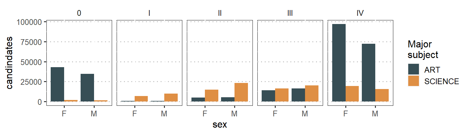
Figure 1: Number of candidate major either in sciene and arts subjects based on gender
References
Firke, Sam. 2020. Janitor: Simple Tools for Examining and Cleaning Dirty Data. https://CRAN.R-project.org/package=janitor.
Rubba, Christian. 2016. Htmltab: Assemble Data Frames from Html Tables. https://CRAN.R-project.org/package=htmltab.
Wickham, Hadley. 2017. Tidyverse: Easily Install and Load the ’Tidyverse’. https://CRAN.R-project.org/package=tidyverse.
———. 2019. Stringr: Simple, Consistent Wrappers for Common String Operations. https://CRAN.R-project.org/package=stringr.
Wickham, Hadley, and Jennifer Bryan. 2018. Readxl: Read Excel Files. https://CRAN.R-project.org/package=readxl.
Wickham, Hadley, Romain François, Lionel Henry, and Kirill Müller. 2018. Dplyr: A Grammar of Data Manipulation. https://CRAN.R-project.org/package=dplyr.
Wickham, Hadley, and Lionel Henry. 2018. Tidyr: Easily Tidy Data with ’Spread()’ and ’Gather()’ Functions. https://CRAN.R-project.org/package=tidyr.