introduction
Time series analysis comprises methods for predicting the future based on the historical in order to extract meaningful statistics and other characteristics of the data. In other words, time series forecasting is the use of a model to predict future values based on previously observed values. Time series are widely used for non-stationary data, like economic, weather, stock price, and retail sales in this post. Scientists all over the globe are also working to predict the future increase of environmenal variables like surface current, wind speed and direction, sea surface temperature and marine productivity. In this post I demonstrate how ot predict chlorophyll concentration in the Pemba channel using prophet package developed by Sean Taylor and Ben Letham (2019).
Let’s get started by loading the package we need to import the data, analyse and plotting:
require(tidyverse)
require(lubridate)
require(magrittr)
require(prophet)
Data
We use a time series of chlorophyll concentration at the Pemba Channel, Tanzania. We extracted these data using the xtracto_3D() function from xtractomatic package (Mendelssohn 2018). The .csv format of this file is available here. First we import the data into our workspace:
chl.tb = read_csv("./chl_tb.csv")The file contain four variables described as:
datethe month of recordslongitudethe eastings geographical coordinates valueslatitudethe northings geographical cooridnates valueschlorophyllthe value of chlorophyll measured at that location and time
| Date | Longitude | Latitude | Chlorophyll (mg/m3) |
|---|---|---|---|
| 2005-10-16 | 40.10 | -5.65 | 0.14 |
| 2005-05-16 | 38.90 | -5.48 | NaN |
| 2011-12-16 | 39.19 | -5.60 | 0.27 |
| 2017-11-16 | 39.27 | -5.56 | 0.20 |
| 2018-03-16 | 39.73 | -5.65 | 0.13 |
| 2004-12-16 | 39.98 | -5.44 | 0.08 |
| 2007-03-16 | 39.19 | -5.65 | 0.37 |
| 2004-05-16 | 39.35 | -5.65 | NaN |
| 2017-05-16 | 39.77 | -5.65 | 0.17 |
| 2017-08-16 | 39.94 | -5.44 | 0.20 |
Data processing
This step includes removing longitude and latitude value from the dataset and aggregate chlorophyll-value by date with function from tidyverse (Wickham 2017). The average chlorophyll concentration was computed and rename the variables to ds for date and date time and y for a variable containing the values to match the data frame format that is compartible with the prophet package (Taylor and Letham 2019).
chl.mean = chl.tb %>%
  group_by(date) %>%
  summarise(chl = mean(chl, na.rm = TRUE)) %>%
  ungroup() %>%
  rename(ds = date, y = chl)
Forecasting
Once we have organized the data frame in the format that prophet package understand, We can fit the data frame of into the model.
m = prophet(df = chl.mean,
            weekly.seasonality=TRUE,
            daily.seasonality=TRUE)
We then used the fitted model to create a data frame of the future. For this case we want to predict chlorophyll value for the next ten years, therefore we specify the number of periods to 120 and the frequency to month. The make_future_dataframe() function takes the model object and a number of periods to forecast and produce a suitable dataframe, but also include the historical dates.
future = make_future_dataframe(m = m,
                               periods = 120,
                               freq = "month")
now you have created a future time and have the historical trend, we can predict the value of chlorophyll for pemba channel for the coming years with the predict() function. It output future.chl data frame object with column yhat containing the predicted values (table 2. It has other columns for uncertainity and seasonal components.
future.chl = predict(m, future)| ds | trend | trend_lower | trend_upper | yhat | yhat_lower | yhat_upper |
|---|---|---|---|---|---|---|
| 2018-01-16 | 0.40 | 0.40 | 0.40 | 0.24 | 0.18 | 0.30 |
| 2010-07-16 | 0.36 | 0.36 | 0.36 | 0.26 | 0.20 | 0.33 |
| 2014-03-16 | 0.38 | 0.38 | 0.38 | 0.15 | 0.09 | 0.22 |
| 2005-07-16 | 0.39 | 0.39 | 0.39 | 0.30 | 0.24 | 0.36 |
| 2027-07-16 | 0.45 | 0.43 | 0.47 | 0.35 | 0.29 | 0.42 |
| 2014-06-16 | 0.38 | 0.38 | 0.38 | 0.27 | 0.20 | 0.33 |
| 2013-12-16 | 0.38 | 0.38 | 0.38 | 0.16 | 0.10 | 0.22 |
| 2023-06-16 | 0.43 | 0.42 | 0.43 | 0.30 | 0.24 | 0.36 |
| 2022-04-16 | 0.42 | 0.42 | 0.43 | 0.27 | 0.21 | 0.33 |
| 2010-12-16 | 0.36 | 0.36 | 0.36 | 0.14 | 0.08 | 0.20 |
Visualize the forecasted values
The generic plot() function can be ussed to plot the predicted chlorophyll value. Note that the model must be supplied in as the first argument and the predicted as the second argument. The nice things is that it uses the ggplot2 framework of grammar of graphics to make this plot. Hence, we can take full control of the rich function of ggplot2 (Wickham 2016), to customize the plot as seen in figure 1.
plot(m,future.chl) +
  # theme_bw()+
  theme(axis.text = element_text(size = 12), axis.title = element_text(size = 14))+
  scale_y_continuous(breaks = seq(0.1, 0.6, 0.1))+
  labs(x = NULL, y = expression(Chlorophyll~concentration~(mgm^{-3})))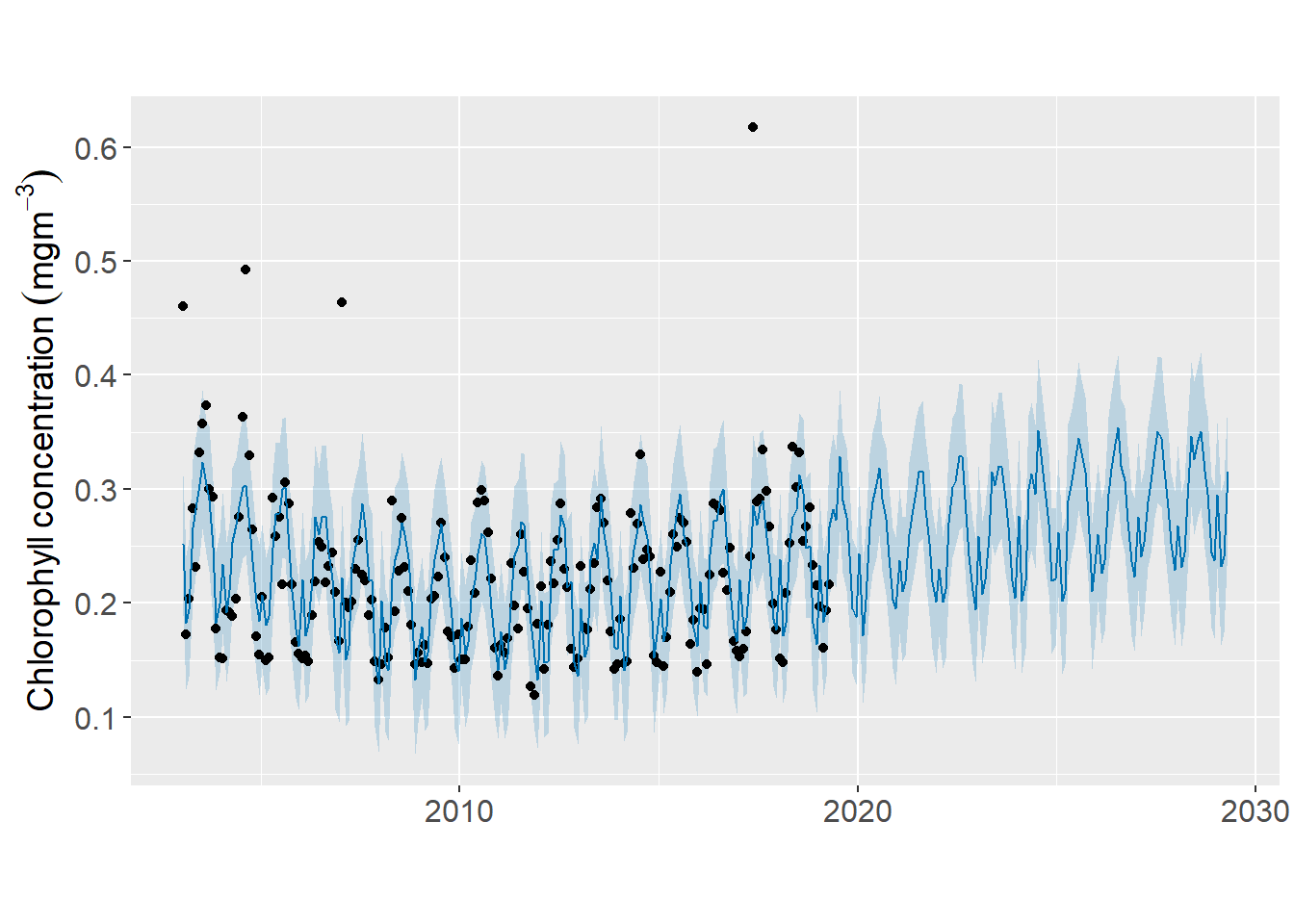
Figure 1: Predicted time series of chlorophyll concentration in the Pemba Channel
We can visualize the components of predicted chlorophyll value shown in figure 2 with the prophet_plot_components() function:
prophet_plot_components(m = m, fcst = future.chl) 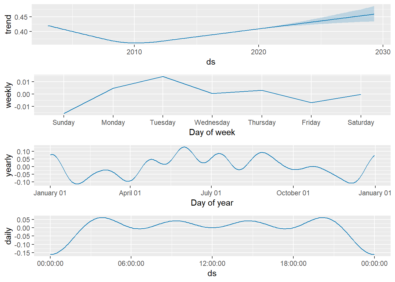
Figure 2: Time series of historical and predicted chlorophyll values decomposed into yearly, week, day and hours trends
We can make an interactive plot of the predicted and historical concentration of chlorophyll as in figure 3 with the dyplot.prophet() function written as;
dyplot.prophet(x = m, fcst = future.chl,uncertainty = TRUE )Figure 3: Interactive plot showing the historical and predicted chlorophyll-value
conclusion
We have seen that with few command line of function from prophet package, we can automatically forecast time series data based on additive models where non-linear trends are unfit. The package works well with time series from the Western Indian Ocean where there is strong effects of monsoon seasons caused by trande winds.
Reference
Mendelssohn, Roy. 2018. Xtractomatic: Accessing Environmental Data from Erd’s Erddap Server. https://CRAN.R-project.org/package=xtractomatic.
Taylor, Sean, and Ben Letham. 2019. Prophet: Automatic Forecasting Procedure. https://CRAN.R-project.org/package=prophet.
Wickham, Hadley. 2016. Ggplot2: Elegant Graphics for Data Analysis. Springer-Verlag New York. http://ggplot2.org.
———. 2017. Tidyverse: Easily Install and Load the ’Tidyverse’. https://CRAN.R-project.org/package=tidyverse.