
tidymodels
tidymodels is a suite of packages that make machine learning with R a breeze. R has many packages for machine learning, each with their own syntax and function arguments. tidymodels aims to provide an unified interface, which allows data scientists to focus on the problem they’re trying to solve, instead of wasting time with learning package syntax.
The tidymodels has a modular approach meaning that specific, smaller packages designed to work hand in hand. Thus, tidymodels is to modeling what the tidyverse is to data wrangling1. The packages included in tidymodels are:
- parsnip for model definition (Kuhn and Vaughan 2020a)
- recipes for data preprocessing and feature engineering (Kuhn and Wickham 2020a)
- rsample to resample data (useful for cross-validation) (Kuhn, Chow, and Wickham 2020)
- yardstick to evaluate model performance (Kuhn and Vaughan 2020b)
- dials to define tuning parameters of your models (Kuhn 2020a)
- tune for model tuning (Kuhn 2020b)
- workflows which allows you to bundle everything together and train models easily (Vaughan 2020)
In this post, I will walk through a machine learning example from start to end and explain how to use the appropriate tidymodels packages at each place. Figure 1 illustrates key modeling steps that are unified in tidymodels that we are going to use use in this article:
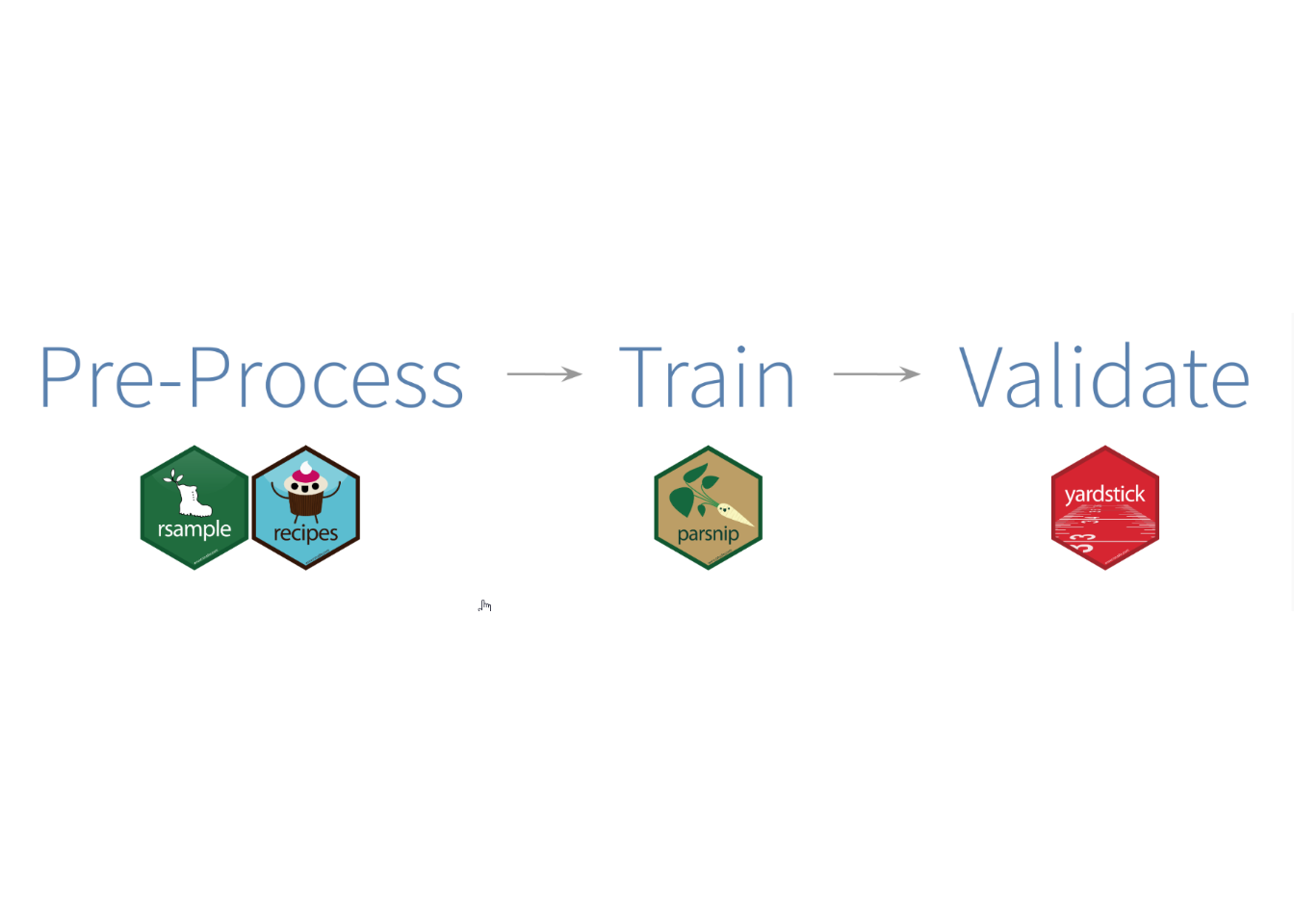
Figure 1: Conceptual model tidymodel’s concept. Courtesy of Edgar Ruiz
After a brief introduction, we proceed with loading some packages we need to work with. We can load the tidymodels (Kuhn and Wickham 2020b) and tidyverse (Wickham 2017) packages into our session. Loading the tidymodels package loads a bunch of packages for modeling and also a few others from the tidyverse like ggplot2 and dplyr. You can use use libray function to load the package, but I prefer require for loading the packages in R.
require(tidymodels)
require(tidyverse)
Data
We use the dagaa dataset to illustrate the concept. This dataset contains 3,869 observations of three variables: species, total length and weight. Speceis is a factor with three levels describing three species of sardines in Lake Tanganyika. We can import the the file using read_csv function from readr package (Wickham, Hester, and Francois 2017).
dagaa.clean = read_csv("dagaa.csv")A quick skim of the dataset reveal that there are three variables (Waring et al. 2020), a Species factor variable and total length and weight of species as numerical variables without missing values. tidymodel prefer string variables as factor and since the Species variable is in factor already, we need no any transformation for now.
dagaa.clean %>%
skimr::skim()| Name | Piped data |
| Number of rows | 3869 |
| Number of columns | 3 |
| _______________________ | |
| Column type frequency: | |
| character | 1 |
| numeric | 2 |
| ________________________ | |
| Group variables | None |
Variable type: character
| skim_variable | n_missing | complete_rate | min | max | empty | n_unique | whitespace |
|---|---|---|---|---|---|---|---|
| species | 0 | 1 | 4 | 5 | 0 | 3 | 0 |
Variable type: numeric
| skim_variable | n_missing | complete_rate | mean | sd | p0 | p25 | p50 | p75 | p100 | hist |
|---|---|---|---|---|---|---|---|---|---|---|
| total_length | 0 | 1 | 80.50 | 36.80 | 33.00 | 64.00 | 77.00 | 85.00 | 480 | ▇▁▁▁▁ |
| weight | 0 | 1 | 7.12 | 27.45 | 0.09 | 1.75 | 2.98 | 4.06 | 707 | ▇▁▁▁▁ |
Figure 2 shows unfit between the points and regression lines of the three species. However, the quadratic fits well the data. This indicates that there is a non–linear relation between total length and weight of the three species, and a higher order terms may solve the problem.
dagaa.clean %>%
  filter(total_length <= 600)%>%
  ggplot(aes(x = total_length, y = weight))+
  geom_jitter(alpha = .2)+
  geom_smooth(method = "lm", formula = "y ~ poly(x, 2)", se = FALSE,
              show.legend = TRUE, aes(color = "Quadratic")) +
  geom_smooth(method = "lm", formula = "y ~ x", se = FALSE,
              show.legend = TRUE, aes(color = "Linear"))+
  facet_wrap(~species, scales = "free")+
  ggpubr::theme_pubclean()+
  scale_color_manual(name = "Model", values = c("blue", "red"))+
  theme(legend.position = "right",
        strip.background = element_blank(),
        legend.key = element_blank())+
  labs(x = "Total length (mm)", y = "Weight of fish (gm)")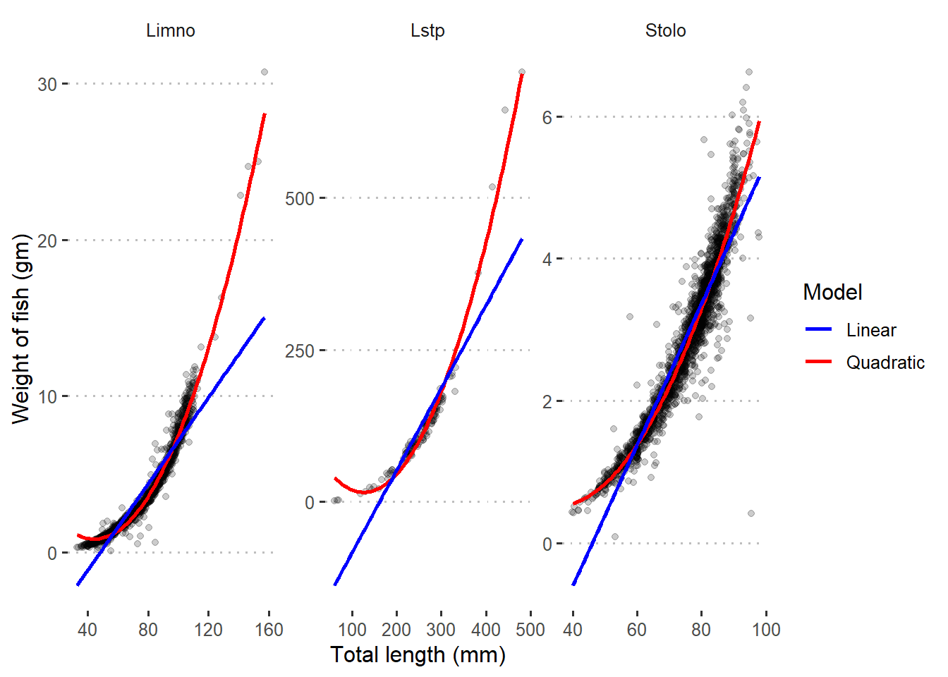
Figure 2: Quadratic and linear regression line superimposed in scatterplot with raw data
Figure 3 indicates that both linear and quadratic models fits well the log–transformed data. This is very clear picture that tell us we need to transform the data before we model them.
dagaa.clean %>%
  ggplot(aes(x = total_length, y = weight))+
  scale_y_continuous(trans = log_trans(), labels = function(x) round(x, -2))+
  scale_x_continuous(trans = log_trans(), labels = function(x) round(x, -2))+
  geom_jitter(alpha = .2)+
  geom_smooth(method = "lm", formula = "y ~ poly(x, 2)",
              se = FALSE, show.legend = TRUE, aes(color = "Quadratic")) +
  geom_smooth(method = "lm", formula = "y ~ x",
              se = FALSE,show.legend = TRUE, aes(color = "Linear"))+
  facet_wrap(~species)+
  ggpubr::theme_pubclean()+
  scale_color_manual(name = "Model", values = c("blue", "red"))+
  theme(legend.position = "right",
        strip.background = element_blank(),
        legend.key = element_blank())+
  labs(x = "Total length (mm)", y = "Weight of fish (gm)")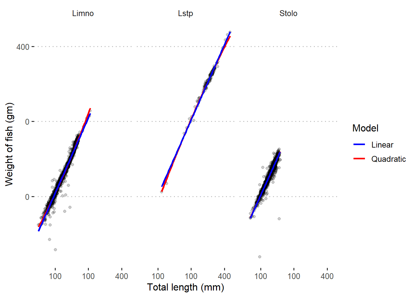
Figure 3: Quadratic and linear regression line superimposed in scatterplot with log-transformed data
We can compute the correlation of total length against weight for each species. The result show a strong correlation coefficient of length and weight for the three species.
dagaa.clean %>% group_by(species) %>%
  summarise(sample = n(),
            correlation = cor(total_length, weight))
# A tibble: 3 x 3
species sample correlation
<chr> <int> <dbl>
1 Limno 1597 0.934
2 Lstp 128 0.863
3 Stolo 2144 0.946We can further test whether the relationship is significant with cor.test function. Because this function does not work in group, I have used a for loop to iterate the process and compute the statistic for each species individually and then stitch them with the bind_rows function.
viumbe = dagaa.clean %>% distinct(species) %>% pull()

cor.stats = list()

for (i in 1:length(viumbe)){

cor.stats[[i]] = dagaa.clean %>%
  filter(species == viumbe[i]) %$%
  cor.test(total_length, weight, method = "pearson") %>%
  broom::tidy() %>%
  mutate_if(is.numeric, round, digits = 2,) %>%
  mutate(Species = viumbe[i])%>%
  select(Species, 2,1,5:6,3 )

}

cor.stats %>% bind_rows()
# A tibble: 3 x 6
Species statistic estimate conf.low conf.high p.value
<chr> <dbl> <dbl> <dbl> <dbl> <dbl>
1 Lstp 19.2 0.86 0.81 0.9 0
2 Stolo 134. 0.95 0.94 0.95 0
3 Limno 104. 0.93 0.93 0.94 0The printed result shows the estimated values (i.e the correlation coefficient), the lower and higher confidence interval and whether the estimated correlation is significant. We see that the length and weight for the three species is strong (R2 > 0.8) ans is significant (p < 0.05). Stolothrissa species have the higher coefficient (R2 > 0.95), compared to Limnothrissa (R2 > 0.93) and Lates (R2 > 0.8).
Pre–Process
Data pre–processing is an important stage in modelling, which clean and transform a raw dataset into useful and understandable format. In layman’s terms, raw data is often incomplete, inconsistent, and might be lacking certain behaviors, and is likely to contain many errors, hence that’s when pre-process comes in.
Data sampling
First, let’s split the dataset into raining and testing set. We will use the training set of iris dataset to train and fit the model and the testing set to evaluate our final model performance. The split is handled automatically using a initial_split function from rsample package (Kuhn, Chow, and Wickham 2020), which creates a special split object.
set.seed(234589)

dagaa.split = dagaa.clean %>%
  rsample::initial_split(prop = .8, strata = "species")
The printed output of iris.split inform us about the number observation we have sampled as trained and testing set along with the total observations.We can extract training and testing sets from the split object using training and testing functions. At a later stage we will tune parameter in the model and hence we want to use a cross-validation object. We also create a cross–validation object from the training set using the vfold_cv function.
## train.set
dagaa.train = dagaa.split  %>%
  rsample::training()

## test set
dagaa.test = dagaa.split %>%
  rsample::testing()

## cross validation set
iris.cv = dagaa.train %>%
  rsample::vfold_cv()
Define a recipe
tidymodels comes with a recipes packages, which provides an interface to specify the role of each variable as either an outcome or predictor using a formula. It also provides pre–processing functions for transforming raw data.
Creating a recipe object with tidymodels package involve two steps chained with pipes. These steps include;
- Specify the formula—specify the formula that feed the predictor and outcome variables
- Specify steps— you specify data transformation steps. Each data transformation is a step. Functions corresponding to specific types of steps has a prefix
step_. recipes has severalstep_*functions.
Looking on figure 4, we notice that weight and total length of the three species varies.
dagaa.clean %>% pivot_longer(cols = 2:3, names_to = "variable", values_to = "data") %>%
  group_by(species, variable) %>%
  summarise(data.mean = mean(data),
            data.sd = sd(data),
            upper = data.mean+data.sd,
            lower = data.mean-data.sd)%>%
  ggplot(aes(x = variable, y = data.mean, col = species)) +
  geom_point(position = position_dodge(.4), size = 4)+
  geom_errorbar(aes(ymin = lower, ymax = upper),
                position = position_dodge(.4), width = .25)+
  ggsci::scale_color_jco(label = c("Limnothrisa","Lates", "Stolothrissa"))+
  ggpubr::theme_pubclean()+
  theme(legend.title = element_blank(), legend.key = element_blank(),
        legend.key.width = unit(2, "lines"), legend.position = "right")+
  coord_cartesian(expand = TRUE) +
  scale_y_continuous(name = "Morphometric", breaks = seq(50,350,50))+
  scale_x_discrete(name = "", labels = c("Total Length (cm)", "Weight (gm)"))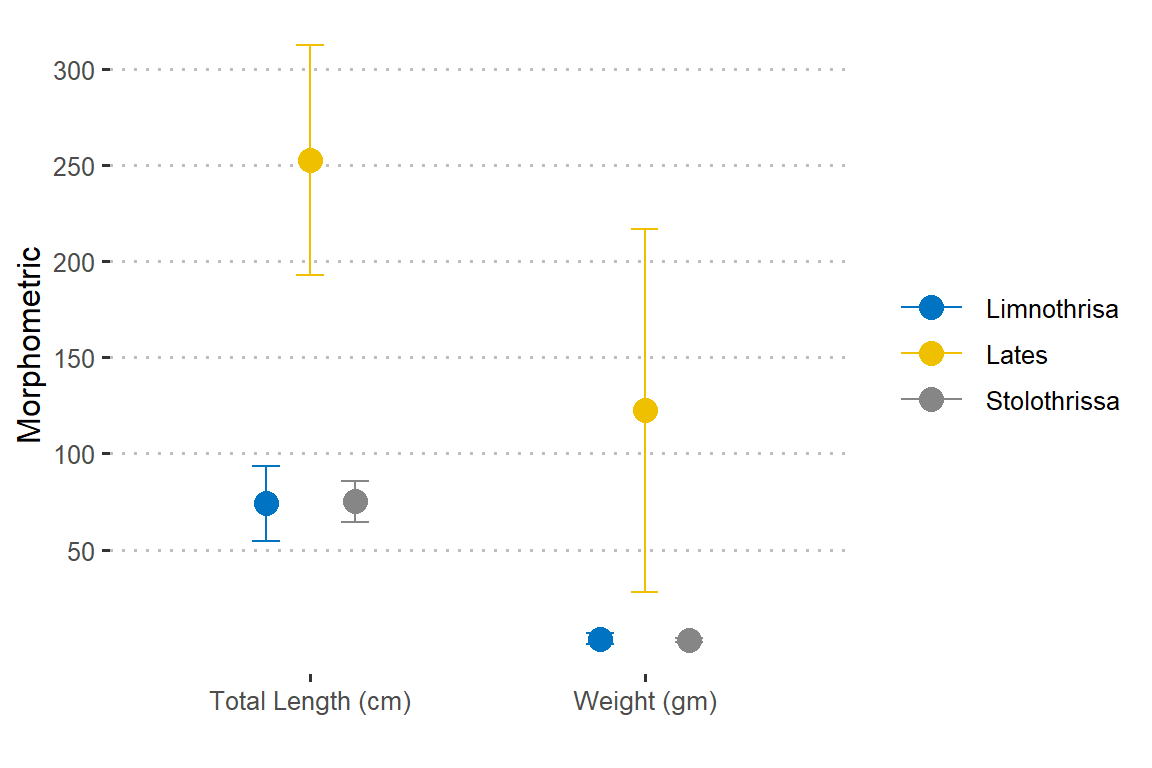
Figure 4: Morphometric measurment of iris flower. The length and width varies for iris flower species
To model them as predictor of species type, we must transform these numeric variables. First, we use step_corr to check the correlation of predictor variables and if two or more variables correlate, others are dropped and one is retained. Then, use the step_normalize to scale and center total length and weight numeric data to have a standard deviation of one.
Other important feature is that we can apply step to a specific variable, groups or all variables in the dataset. The all_outcomes and all_predictors functions provide convenient ways to specify groups of variables. For instance, if we want step_normalize to transform only predictors we simply parse step_corr(all_predictors()).
After a brief introduction of recipe, we can now go on and create a recipe object. We use the training set and not the raw iris dataset to define the following recipe, transform and prep.
dagaa.recipe = dagaa.train %>%
  recipe(species ~ .) %>%
  step_normalize(all_numeric()) %>%
  # step_dummy(sex, stage_mat) %>%
  step_corr(all_numeric()) %>%
  prep()
You notice that I have specified the short formula species ~ ., where . represents all variable in the dataset. If we are interested with the recipe object we just created, we can simply print it in a console.
dagaa.recipeData Recipe
Inputs:
role #variables
outcome 1
predictor 2
Training data contained 3096 data points and no missing data.
Operations:
Centering and scaling for total_length, weight [trained]
Correlation filter removed no terms [trained]The printed output describes what was done and the how many variables are used as outcome and predictor. It also tells us that the step_corr there is no auto correlation of the variable. We can further extracted the transformed testing dataset from prepped and recipe data data with the juice function. Note that a transformed dagaa.training must originate from the recipe, which is prepped.
## transformed training set
dagaa.training = dagaa.recipe %>%
  juice()

dagaa.training %>% glimpse()
Rows: 3,096
Columns: 3
$ total_length <dbl> -0.3398847, -0.2552734, -0.5373111, 5.7521316, 5.07524...
$ weight <dbl> -0.1851922, -0.1896358, -0.2070400, 5.3789633, 4.34322...
$ species <fct> Lstp, Lstp, Lstp, Lstp, Lstp, Lstp, Lstp, Lstp, Lstp, ...We also need to transform the testing set of the dagaa dataset. We can do that by parsing the dagaa.test data set we extracted from the dagaa.split in a bake function. Note that the transformation of the iris.testing must originate from the recipe, which is prepped and recipe dagaa.test` set.
## transformed testing set
dagaa.testing = dagaa.recipe %>%
  recipes::bake(dagaa.test)

dagaa.testing %>% glimpse()
Rows: 773
Columns: 3
$ total_length <dbl> 5.188056, 5.780335, 5.244464, 4.257331, 4.652184, 5.27...
$ weight <dbl> 4.605773, 5.321196, 4.282129, 2.792775, 3.621511, 3.71...
$ species <fct> Lstp, Lstp, Lstp, Lstp, Lstp, Lstp, Lstp, Lstp, Lstp, ...Train a model
So far we have split the dataset into training and testing, we have create a prepped recipe object, extracted transformed training set and transformed the testing set. The next step we need to do is to train our model using the parsnip package (Kuhn and Vaughan 2020a). parsnip provides a unified interface of different models that exist in R.
There are a few primary components that you need to provide for the model specification. These includes;
- Model type specify a function that define a model like
rand_forestfor random forest andlogistic_regfor logistic regression. If you are wondering of type of modes to use, you can consult this article that describe different function tidymodels support - Set arguments are set using
set_args - Set engine is the specific package that the model you choose must come from. For instance the
rangerengine drives the Random Forest model andglmnetdrives the Logistic regression. You specify the engine to use in the model with theset_enginefunction. - Set mode allows to specify the type of prediction—whether
classificationfor binary/categorical prediction orregressionfor continuous prediction.
For instance, if we want to fit a random forest model as implemented by the ranger package for the purpose of classification, the rand_forest() function is used to initialize a Random Forest model and parse the trees argument to define number of tree. Then we use set_engine() function to command rand_forestfunction for Random Forest model we specified must come fromrangerpackage. Since the prediction is binary, we used theset_modeto specify the type of model. Finally, to execute the model, thefit()` function is used.
This will automatically train the model specified using the transformed training data. Notice that the model runs on top of the juiced trained data because is a transformed instead of the raw trained. The chunk below shows the model specification.
rf.model = rand_forest() %>%
  set_engine(engine = "ranger") %>%
  set_mode(mode = "classification") %>%
  fit(species~., data = dagaa.training)

rf.model
parsnip model object
Fit time: 720ms
Ranger result
Call:
ranger::ranger(formula = formula, data = data, num.threads = 1, verbose = FALSE, seed = sample.int(10^5, 1), probability = TRUE)
Type: Probability estimation
Number of trees: 500
Sample size: 3096
Number of independent variables: 2
Mtry: 1
Target node size: 10
Variable importance mode: none
Splitrule: gini
OOB prediction error (Brier s.): 0.1553012 Note that the printed fit object provide the model result.
Metrics To Evaluate Classification Model
The yardstick package is specifically designed to measure model performance for both numeric and categorical outcomes, and it plays well with grouped predictions. A nice thing about tidymodels is that when we use predict function in the fitted model against the transformed testing set, the output is the tibble.
Accuracy and Kappa
Accuracy is the percentage of correctly classifies instances out of all instances. It is more useful on a binary classification than multi-class classification problems because it can be less clear exactly how the accuracy breaks down across those classes (e.g. you need to go deeper with a confusion matrix). Learn more about Accuracy here.
Kappa or Cohen’s Kappa is like classification accuracy, except that it is normalized at the baseline of random chance on your dataset. It is a more useful measure to use on problems that have an imbalance in the classes (e.g. 70-30 split for classes 0 and 1 and you can achieve 70% accuracy by predicting all instances are for class 0).
since all the prediction information is tibble, we can apply the metric function from yardstick and compare original species value (truth = Species) against predicted species values (estimate = .pred_class) to evaluate our model performance. The function expects a tibble that contains the actual results (truth) and what the model predicted (estimate). The metrics() function calculates accuracy and kap metrics for numeric outcomes. Furthermore, it automatically recognizes that lm_preds is grouped by folds and thus calculates the metrics for each fold.
rf.model %>% predict(dagaa.testing) %>%
  bind_cols(dagaa.testing) %>%
  metrics(truth = species, estimate = .pred_class)
# A tibble: 2 x 3
.metric .estimator .estimate
<chr> <chr> <dbl>
1 accuracy multiclass 0.771
2 kap multiclass 0.570The printed output indicates that our model has an accuracy of 0.77 andd the kappa of 0.56.
Gain and Roc Curve
When we develop statistical models for classification tasks (e.g. using machine learning), we usually need to have a way to compare the generated models results to help us decide whether the model fitted well the data—the best model. Some of the tools in yardstick package include gains and `roc1 tools.
The Gains and the ROC curve are visualizations showing overall performance of the models. The shape of the curves will tell us a lot about the behavior of the model. It clearly shows how much our model is better than a model assigning categories randomly and how far we are from the optimal model which is in practice unachievable. These curves can help in setting the final cut-off point for deciding which probabilities will mean positive and negative response prediction.
In order to plot gain or roc curve, we need first to compute the probability for each possible predicted value by setting the type argument to prob. That will return a tibble with as many variables as there are possible predicted values. Their name will default to the original value name, prefixed with .pred_.
dagaa.prob = rf.model %>%
  predict(dagaa.testing, type = "prob") %>%
  bind_cols(dagaa.testing)
Gain Curve
Once we have the probability of prediction, we can use gain_curve function fro yardstick package to compute values for gain curve. Figure 5 is a gain plot. The gains associated with the model is shown as black curve for the three species.
dagaa.gain = dagaa.prob %>%
  yardstick::gain_curve(species,
                        .pred_Limno,
                        .pred_Lstp,
                        .pred_Stolo)

dagaa.gain %>%
  autoplot()+
  ggpubr::theme_pubclean()+
  theme(strip.background = element_blank())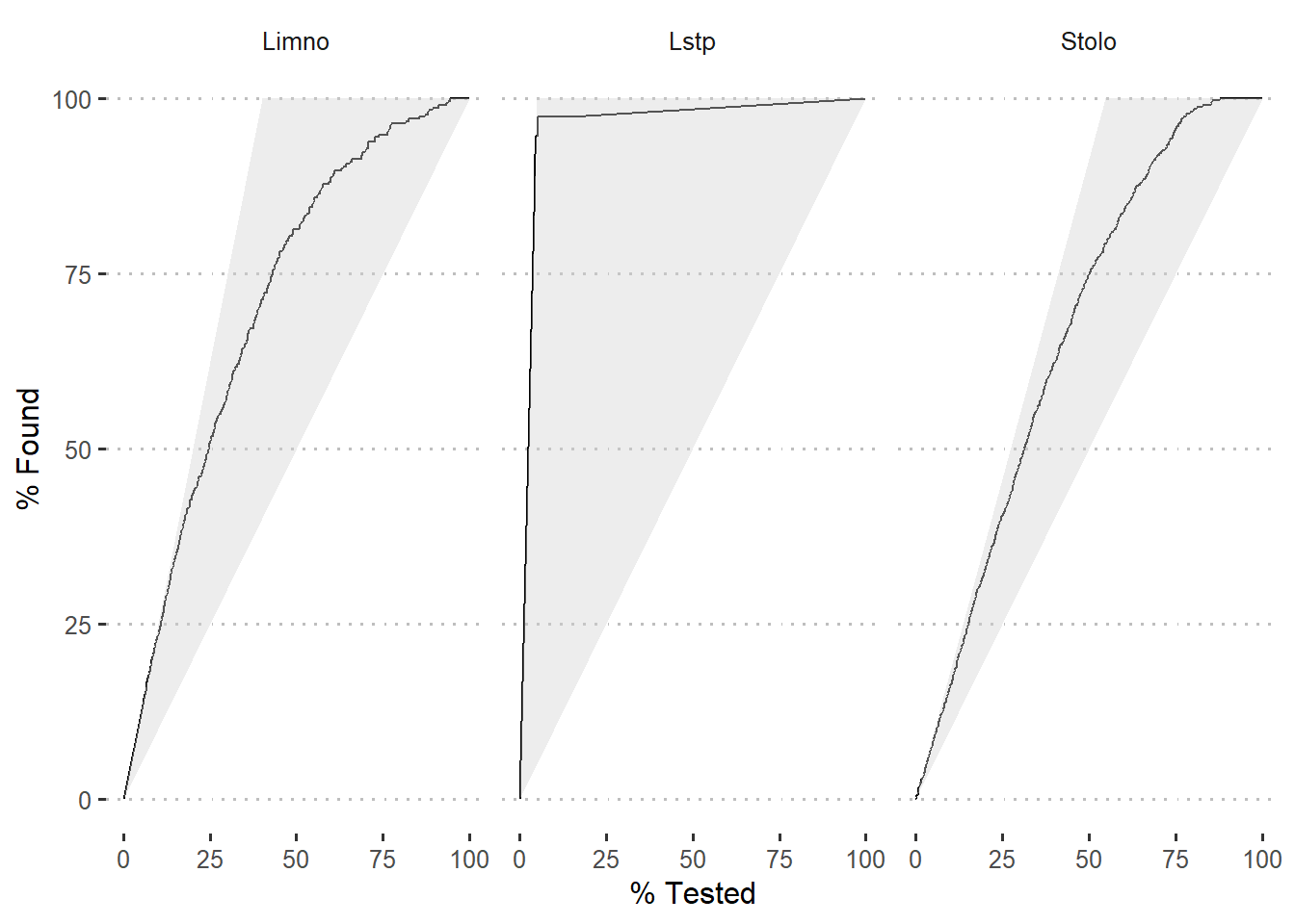
Figure 5: Gain curve of modelled species
ROC curve
The other tool used to assess the model accuracy based on a confusion matrix are Sensitivity and Specificity. The ROC curve (Receiver Operating Characteristics curve) is the display of sensitivity and specificity for different cut-off values for probability (If the probability of positive response is above the cut-off, we predict a positive outcome, if not we are predicting a negative one). Each cut-off value defines one point on ROC curve, ranging cut-off from 0 to 1 will draw the whole ROC curve. to obtain the value for roc curve, we use the roc_curve function from yardstick.
dagaa.roc = dagaa.prob %>%
  yardstick::roc_curve(species,
                        .pred_Limno,
                        .pred_Lstp,
                        .pred_Stolo)
The black curve on ROC curve in figure 6 is the same model as the example for the Gains chart (Figure 5). The Y axis measures the rate (as a percentage) of correctly predicted species with a positive response. The X axis measures the rate of incorrectly predicted species with a negative response. Since the optimal model should have sensitivity that rise to a maximum and specificity will stay the whole time at 1. The task is to have ROC curve of the developed model as close as possible to optimal model. Therefore, based on that information, figure 6 indicates that our model predicted well for Lates species as compared to Limno and Stolo.
dagaa.roc %>%
  autoplot()+
  ggpubr::theme_pubclean()+
  theme(strip.background = element_blank())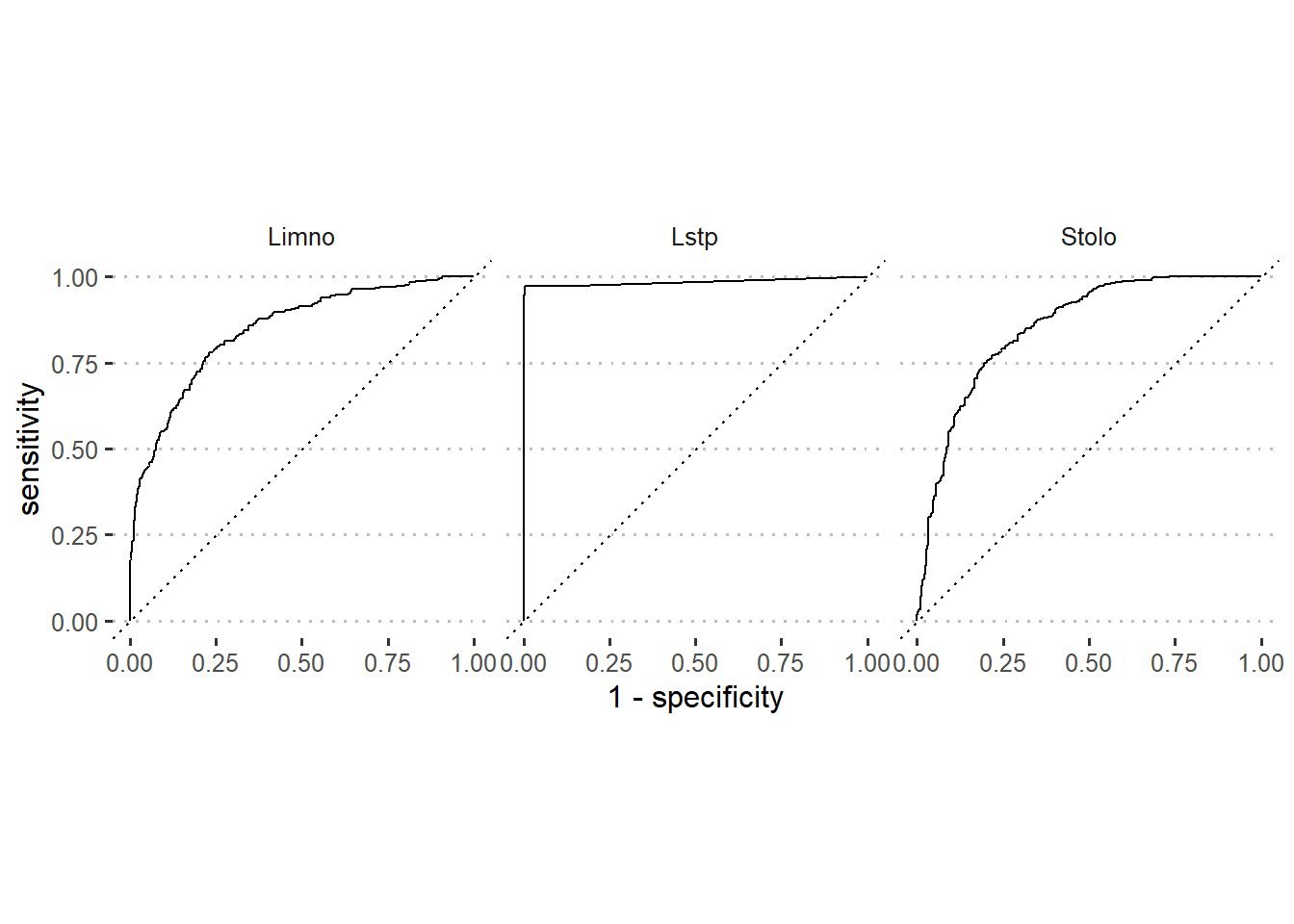
Figure 6: Roc curve of modelled species
Summary
I hanged on Rebecca Barter post on Tidymodels: tidy machine learning in R that explain briefly the use of tidymodels package in R. I also glimpsed Edger Ruiz post that provide a gentle introduction to tidymodels. These post provided resourceful material for learning basic functions of tidymodels.
References
Kuhn, Max. 2020a. Dials: Tools for Creating Tuning Parameter Values. https://CRAN.R-project.org/package=dials.
———. 2020b. Tune: Tidy Tuning Tools. https://CRAN.R-project.org/package=tune.
Kuhn, Max, Fanny Chow, and Hadley Wickham. 2020. Rsample: General Resampling Infrastructure. https://CRAN.R-project.org/package=rsample.
Kuhn, Max, and Davis Vaughan. 2020a. Parsnip: A Common Api to Modeling and Analysis Functions. https://CRAN.R-project.org/package=parsnip.
———. 2020b. Yardstick: Tidy Characterizations of Model Performance. https://CRAN.R-project.org/package=yardstick.
Kuhn, Max, and Hadley Wickham. 2020a. Recipes: Preprocessing Tools to Create Design Matrices. https://CRAN.R-project.org/package=recipes.
———. 2020b. Tidymodels: Easily Install and Load the ’Tidymodels’ Packages. https://CRAN.R-project.org/package=tidymodels.
Vaughan, Davis. 2020. Workflows: Modeling Workflows. https://CRAN.R-project.org/package=workflows.
Waring, Elin, Michael Quinn, Amelia McNamara, Eduardo Arino de la Rubia, Hao Zhu, and Shannon Ellis. 2020. Skimr: Compact and Flexible Summaries of Data. https://CRAN.R-project.org/package=skimr.
Wickham, Hadley. 2017. Tidyverse: Easily Install and Load the ’Tidyverse’. https://CRAN.R-project.org/package=tidyverse.
Wickham, Hadley, Jim Hester, and Romain Francois. 2017. Readr: Read Rectangular Text Data. https://CRAN.R-project.org/package=readr.