I was looking for bathymetry dataset for Lake Victoria online and I came across this link. It stores several products of the bathymetry data of the Lake Victoria. Among them products is the gridded TIFF file. This dataset was created by a team from Harvard University in 2017 (Hamilton et al. 2016). They used over 4.2 million points collected over 100-years of surveys. The point data was obtained from an Admiral Bathymetry map and points collected in the field. Roughly, 3.8 million points come from the survey conducted by Lake Victoria Regional Hydro-acoustics Working Group.
In this post I illustrate step by step processing the bathymetric of Lake Victoria, which is stored in n TIFF format using R language (R Core Team 2018). You first need to download the dataset from here as TIFF. It has about 48 MB, so you need to patient if you internet speed is slow for this file to download. I load some of the packages to manipulate, analyse and even visualize the bathymetry data of Lake Victoria. These packages include;
require(tidyverse)
require(sf)
require(leaflet)
raster package contains nifty function to handle raster file like the bathymetry dataset of Lake Victoria (Hijmans 2017). But, often there conflict between raster and tidyverse packages, I will only call specific function of raster package when needed using the raster:: arguments throughtout this post. Once the dataset is download, you can simply load or import in R session using raster function from raster package (Hijmans 2017).
## read the ascii file
lake.victoria = raster::raster("e:/GIS/Lake_victoria/LV_Bathy_V7.tif")

lake.victoria.shp = st_read("e:/GIS/Lake_victoria/wb_lv_tzn.shp", quiet = TRUE)
When we plot the bathymetry of Lake Victoria as shown in figure 1, we notice that depth vary across the lake range between 0 to about 80 meters deep. Unfortunately, the longitude and latitude values are unfamiliar to me and I the datum used to present this dataset are unclear to me.
lake.victoria %>% raster::plot()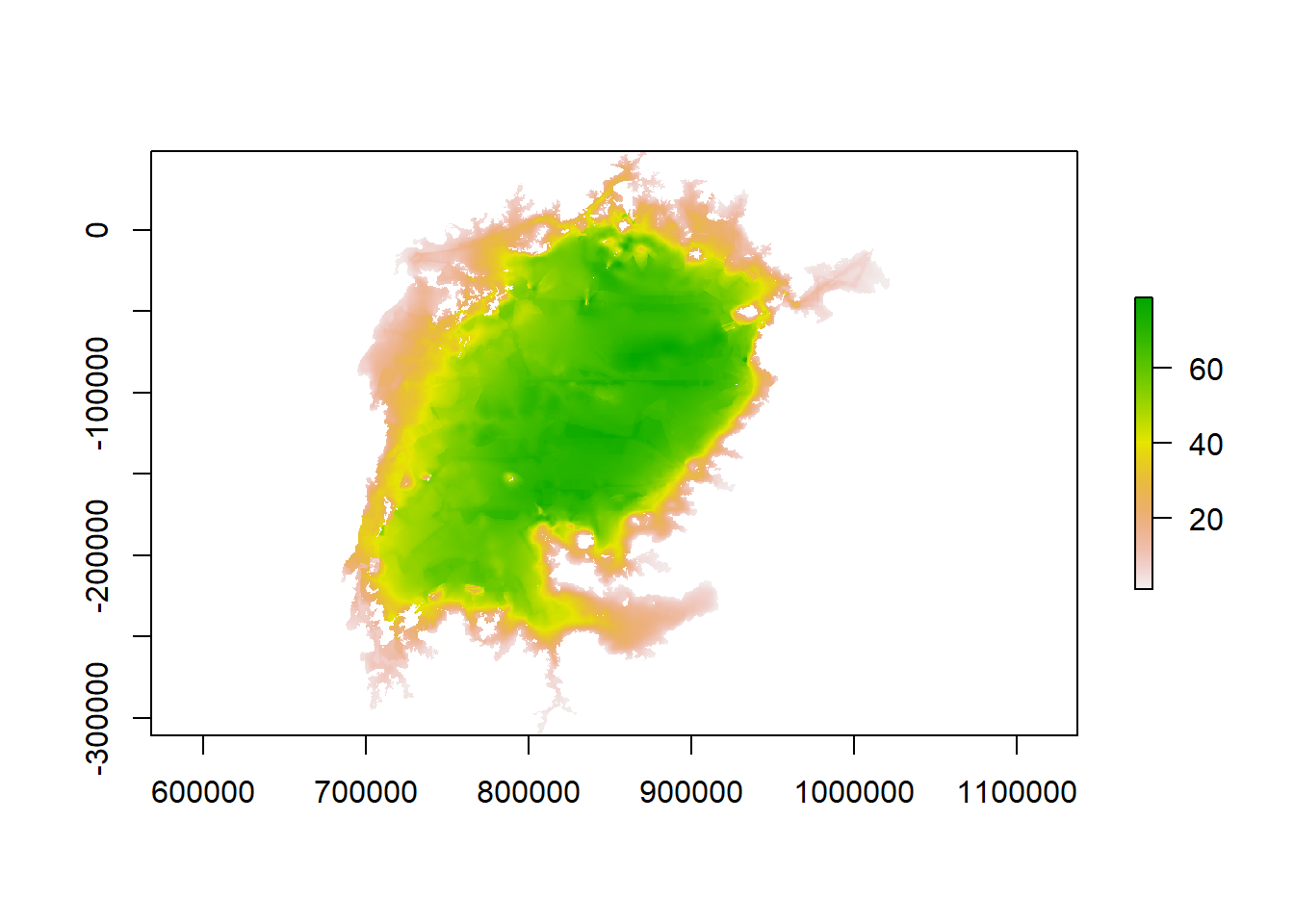
Figure 1: Lake Victoria batymetry map
To have a glimpse of the Coordinate Reference System (CRS) in the dataset, I used raster::crs() function to check the datum used;
lake.victoria %>% raster::crs()FALSE CRS arguments:
FALSE +proj=lcc +lat_1=20 +lat_2=-23 +lat_0=0 +lon_0=25 +x_0=0 +y_0=0
FALSE +datum=WGS84 +units=m +no_defs +ellps=WGS84 +towgs84=0,0,0Reproject Rasters
We can use the projectRaster function to reproject a raster into a new CRS. I have used +proj=longlat +ellps=WGS84 +datum=WGS84 to transform the projection into WGS84 geographical coordinate system of longitude and latitude measured in degree. Keep in mind that reprojection only works when you first have a defined CRS for the raster object that you want to reproject.
# reproject to UTM
lake.victoria.wgs = lake.victoria %>%
  raster::projectRaster(crs="+proj=longlat +ellps=WGS84 +datum=WGS84")
When we replot the projected bathymetry as shown in figure 2, we notice that the longitude and latitude are in degree.
lake.victoria.wgs %>% raster::plot()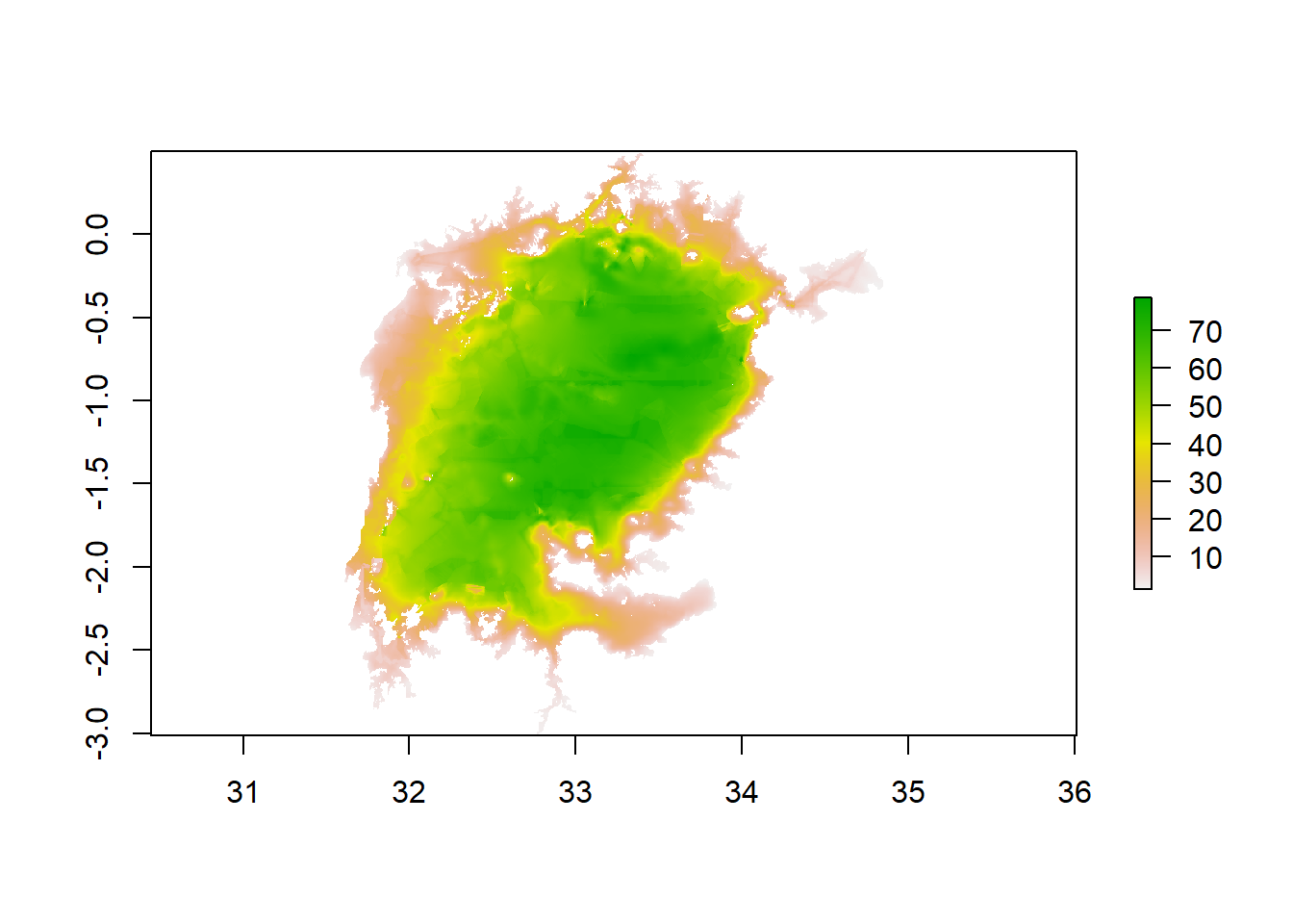
Figure 2: Transformed projection of Lake Victoria bathymetry to datum WGS84
If we are fine with the projection, but the plotting isn’t pleasing. We might want to use the grammar of graphic ggplot2 and its extended package like the metR to improve the plot. However, these package use data organized in data frame instead of raster. We use the raster::as.data.frame(xy = TRUE) to convert raster to data frame and tidy the data into lon, lat, and depth with rename(lon = x, lat = y, depth = 3) from dplyr package (Wickham et al. 2018).
## convert raster to data frame
lake.victoria.df = lake.victoria.wgs %>%
  raster::as.data.frame(xy = TRUE) %>%
  dplyr::as_tibble() %>%
## rename the variable
  dplyr::rename(lon = x, lat = y, depth = 3)%>%
  dplyr::mutate(depth = as.numeric(depth))
Once we have organized the data frame from raster, we can use the information now to plot the spatial variation of water depth in the lake. Figure 3 show filled contour of depth in Lake Victoria. This figure 3 was plotted using the code in the chunk below;
lake.victoria.df %>%
  ggplot(aes(x = lon, y = lat))+
  geom_contour_filled(aes(z = depth))+
  metR::scale_x_longitude(ticks = 0.5)+
  metR::scale_y_latitude(ticks = 0.5)+
  coord_cartesian(expand = FALSE)+
  theme(panel.background = element_blank(), panel.grid = element_line(linetype = 3))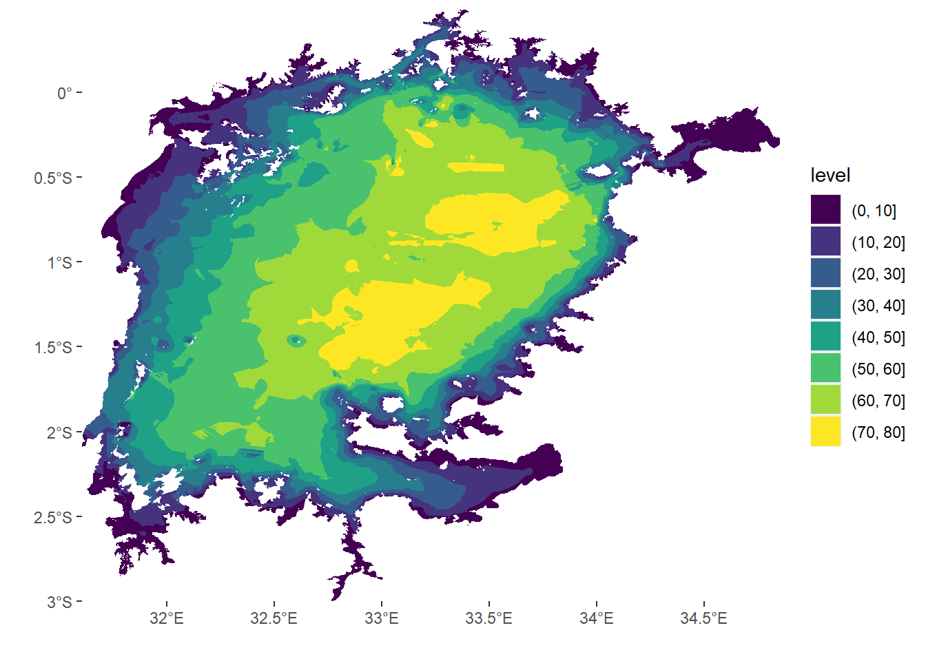
Figure 3: Bathymetry of Lake Victoria
We may also wish to plot only the section of the lake and use contour lines instead of filled contour. we need then to have base maps. the chunk below show how to import the base maps into our session. The lake boundary is in projected in UTM zone 36 south and the regions layer is in WGS84. Therefore, I will import and project on the fly the lake baseman, but for the region baseman simply import into the session with the st_read function (Pebesma 2018). To reduce processing time while drawing contour, the lake baseman data frame was filter to accommodate only value that fall within the specified area of interest using filter function from dplyr (Wickham et al. 2018)
## import lake boundary and project to wgs84
lv.boundary = st_read("e:/GIS/Lake_victoria/wb_lv_tzn.shp", quiet = TRUE) %>%
  st_transform(4326)

## import basemap contain regions in Tanzania
boundary = st_read("e:/GIS/tanzania-latest.shp/nbs/Districts.shp", quiet = TRUE)

## chop the area of interest
mwanza.gulf= lake.victoria.df %>%
  dplyr::filter(lon > 33.25 & lon < 34 &
                  lat > -2.0 & lat < -1.5)
I then plot the contour shown in figure 4 using the combination of ggplot2 (Wickham 2016) and metR (Campitelli 2019) packages. The chunk below highlight the code used to plot figure figure 4
  ggplot()+
  # geom_sf(data = lv.boundary, fill = NA, col = "black", size = .5) +
  metR::geom_contour2(data = mwanza.gulf, aes(x = lon, y = lat, z = depth),
                      binwidth = 5, col = "grey60", size = 0.25)+
  metR::geom_text_contour(data = mwanza.gulf, aes(x = lon, y = lat, z = depth),
                          binwidth = 5, stroke = .80,
                          stroke.color = "white", check_overlap = TRUE,
                          col = "grey50", rotate = FALSE, parse = TRUE, size = 3.2)+
  geom_sf(data = boundary, col = "#ED6300", fill = "#FBE1CB",size = .5) +
  metR::scale_x_longitude(breaks = c(33.35,33.68))+
  metR::scale_y_latitude(breaks = c(-1.81,-1.58))+
  coord_sf(expand = FALSE, ylim = c(-1.85, -1.55), xlim = c(33.3,33.73))+
  theme_bw()+
  theme(panel.background = element_rect(fill = NA, colour = "black"),
        panel.grid = element_line(linetype = 3), axis.text = element_text(size = 11))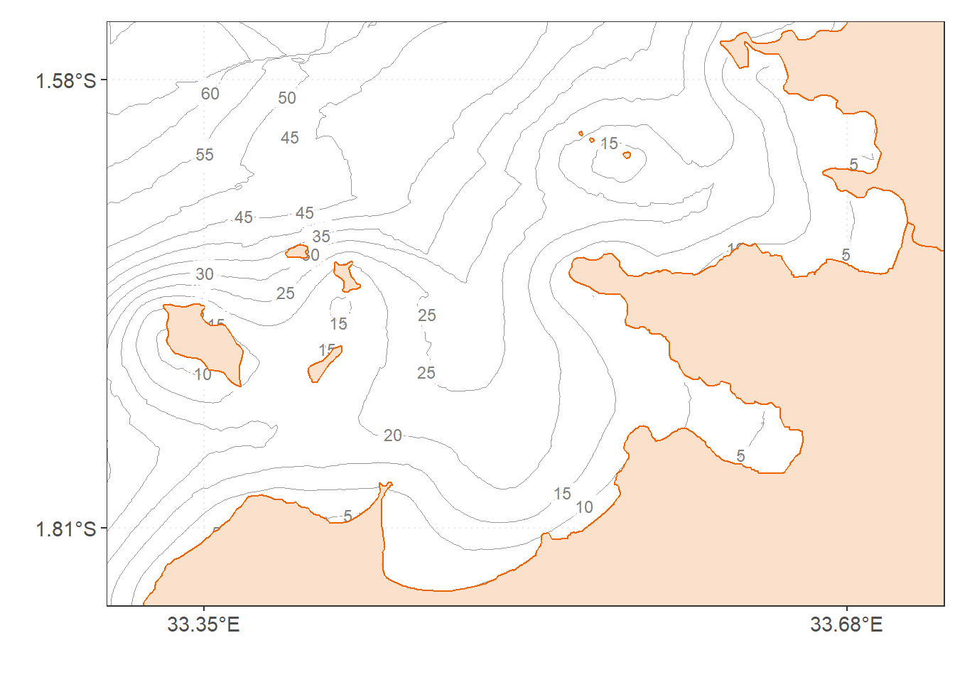
Figure 4: Contour map in Lake Victoria
Extracting information from bathymetric data
Although there several function to extract value from the raster package, in this post we will use extract() function from raster package to retrieve depth information on a set of longitude/latitude pairs. This is helpful to get depth information along a GPS track record for instance. Table 1 show stations and pairs of longitude and latitude. We will use these geographical positions in this dataset to extracts depth.
| Station | Longitude | Latitude |
|---|---|---|
| E | 32.89067 | -2.568583 |
| F | 32.88360 | -2.561467 |
| G | 32.87533 | -2.555717 |
| H | 32.86427 | -2.551117 |
| I | 32.85027 | -2.549017 |
| J | 32.84070 | -2.546917 |
Before we extract, we need to convert spatial information in table 1 to simple feature; You can do that using the st_as_sf function from *sf** package (Pebesma 2018). The process of turning spatial information in tabular form into spatial feature is highlighted in the chunk below;
gulf.sf = gulf.tb %>%
  st_as_sf(coords = c("lon", "lat")) %>%
  st_set_crs(4326)
We can then extract the depth from the raster layer at the corresponding pair of latitude and longitude using the extract function of raster package. You must make sure that the raster and simple feature layers that you intend to use for extraction are in the same projections. The result of the extraction is a vector with depth value, which you then combine with the original dataset (Table 2). The chunk below show the two main steps explained above;
## extract points to a specific geographical location
depth = lake.victoria %>%
  raster::extract(gulf.sf) %>% as_tibble()

## bind the depth to the dataset
gulf.tb = gulf.tb %>% bind_cols(depth) %>%
  rename(depth = value) %>%
mutate_if(is.numeric, round, digits = 3)| Station | Longitude | Latitude | Depth [m] |
|---|---|---|---|
| E | 32.891 | -2.569 | 12.003 |
| F | 32.884 | -2.561 | 14.273 |
| G | 32.875 | -2.556 | 15.853 |
| H | 32.864 | -2.551 | 14.615 |
| I | 32.850 | -2.549 | 8.888 |
| J | 32.841 | -2.547 | 6.650 |
You might need to customize the information you want to visualize on the interactive map like leaflet. For instance, i want to show the depth extracted in section ?? and the corresponding information shown in table 2 as table in leaflet. To do that, I must add a column label with html tag. Therefore, the function below will add the label variable as html table in the dataset, which is then used to display the information in the interactive map shown in figure ?? label with the
## label for leaflet popups
library("htmltools")

addLabel <- function(data) {

  data$label <- paste0(
    '<b>',  '</b><br>
    <table style="width:120px;">
    <tr><td>Station:</td><td align="right">', data$station, '</td></tr>
    <tr><td>Longitude:</td><td align="right">', data$lon, '</td></tr>
    <tr><td>Latitude:</td><td align="right">', data$lat, '</td></tr>
    <tr><td>Depth:</td><td align="right">', data$depth, '</td></tr>
    </table>'
  )
  data$label <- lapply(data$label, HTML)

  return(data)
}

gulf.tb = gulf.tb %>% addLabel()
Figure 5: The map showing the positions of the sampled locations across the Mwanza Gulf. To view the name of the marks on the map and other information just click any mark
Cited references
Campitelli, Elio. 2019. MetR: Tools for Easier Analysis of Meteorological Fields. https://CRAN.R-project.org/package=metR.
Hamilton, Stuart, Anthony Taabu Munyaho, Noah Krach, and Sarah Glaser. 2016. “Bathymetry TIFF, Lake Victoria Bathymetry, raster, 2017, V7.” Harvard Dataverse. https://doi.org/10.7910/DVN/SOEKNR.
Hijmans, Robert J. 2017. Raster: Geographic Data Analysis and Modeling. https://CRAN.R-project.org/package=raster.
Pebesma, Edzer. 2018. Sf: Simple Features for R. https://CRAN.R-project.org/package=sf.
R Core Team. 2018. R: A Language and Environment for Statistical Computing. Vienna, Austria: R Foundation for Statistical Computing. https://www.R-project.org/.
Wickham, Hadley. 2016. Ggplot2: Elegant Graphics for Data Analysis. Springer-Verlag New York. http://ggplot2.org.
Wickham, Hadley, Romain François, Lionel Henry, and Kirill Müller. 2018. Dplyr: A Grammar of Data Manipulation. https://CRAN.R-project.org/package=dplyr.