Access, Download, Process and VIsualize sea surface height and geostrophic current from AVISO in R

In this post I explain how to read the NetCDF file of aviso in R. I also showed how to make plot of the processed sea surface height with ggplot2 package (Wickham 2016) and also animated a series of map with gganimate packages (Pedersen and Robinson 2017). However, the link that I used to obtain the data is no longer active and people find difficult to follow the instructions in the post. Therefore, in this post I show how to download the aviso data from the website into R (Mendelssohn 2018).

require(xtractomatic)
require(lubridate)
require(tidyverse)

R has powerful packages that can download data from ERDAPP server. Among the dataset that are public available are product of AVISO. You can use the searchData() function from xtractomatic package to search for a dataset name that you need (Mendelssohn 2018). For example the chunk below highlight how to search dataset name of daily products from ERDAPP server.

# result  = searchData("varname:ssh")
daily.dataset = searchData("datasetname:1day")

The file contains a lot of information, you can have a glimpse of the structure of the file with the glimpse() function from dplyr package (Wickham et al. 2018). This gives a list of the datasetname of the 46 daily products.

daily.dataset %>% glimpse()

Observations: 19
Variables: 46
$ agssta1day               <list> ["agssta1day", "erdAGssta1day", "SST...
$ atssta1day               <list> ["atssta1day", "erdATssta1day", "SST...
$ erdG1ssta1day            <list> ["erdG1ssta1day", "erdG1ssta1day", "...
$ erdGAtfnt1day            <list> ["erdGAtfnt1day", "erdGAtfnt1day", "...
$ erdGRssta1day            <list> ["erdGRssta1day", "erdGRssta1day", "...
$ erdMBsstd1day            <list> ["erdMBsstd1day", "erdMBsstd1day", "...
$ erdMH1pp1day             <list> ["erdMH1pp1day", "erdMH1pp1day", "Pr...
$ erdMWchla1day            <list> ["erdMWchla1day", "erdMWchla1day", "...
$ erdMWpp1day              <list> ["erdMWpp1day", "erdMWpp1day", "Prim...
$ erdMWsstd1day            <list> ["erdMWsstd1day", "erdMWsstd1day", "...
$ erdQAstress1daycurl      <list> ["erdQAstress1daycurl", "erdQAstress...
$ erdQAstress1daymodStress <list> ["erdQAstress1daymodStress", "erdQAs...
$ erdQAstress1daytaux      <list> ["erdQAstress1daytaux", "erdQAstress...
$ erdQAstress1daytauy      <list> ["erdQAstress1daytauy", "erdQAstress...
$ erdQAstress1dayupwelling <list> ["erdQAstress1dayupwelling", "erdQAs...
$ erdQAwind1dayx_wind      <list> ["erdQAwind1dayx_wind", "erdQAwind1d...
$ erdQAwind1dayy_wind      <list> ["erdQAwind1dayy_wind", "erdQAwind1d...
$ erdQAxwind1day           <list> ["erdQAxwind1day", "erdQAwind1day", ...
$ erdQAywind1day           <list> ["erdQAywind1day", "erdQAwind1day", ...
$ erdSHchla1day            <list> ["erdSHchla1day", "erdSHchla1day", "...
$ erdSW1chla1day           <list> ["erdSW1chla1day", "erdSW1chla1day",...
$ erdTAssh1day             <list> ["erdTAssh1day", "erdTAssh1day", "Se...
$ erdTAugeo1day            <list> ["erdTAugeo1day", "erdTAgeo1day", "U...
$ erdTAvgeo1day            <list> ["erdTAvgeo1day", "erdTAgeo1day", "V...
$ erdVH3chla1day           <list> ["erdVH3chla1day", "erdVH3chla1day",...
$ erdVH3k4901day           <list> ["erdVH3k4901day", "erdVH3k4901day",...
$ erdVH3par1day            <list> ["erdVH3par1day", "erdVH3par1day", "...
$ erdVH3pic1day            <list> ["erdVH3pic1day", "erdVH3pic1day", "...
$ erdVH3poc1day            <list> ["erdVH3poc1day", "erdVH3poc1day", "...
$ erdVH3r6711day           <list> ["erdVH3r6711day", "erdVH3r6711day",...
$ erdVHNchla1day           <list> ["erdVHNchla1day", "erdVHNchla1day",...
$ gassta1day               <list> ["gassta1day", "erdGAssta1day", "SST...
$ jplMURSST41anom1day      <list> ["jplMURSST41anom1day", "jplMURSST41...
$ mbchla1day               <list> ["mbchla1day", "erdMBchla1day", "Chl...
$ mhchla1day               <list> ["mhchla1day", "erdMH1chla1day", "Ch...
$ mhsstd1day               <list> ["mhsstd1day", "erdMH1sstd1day", "SS...
$ nodcPH2sstd1day          <list> ["nodcPH2sstd1day", "nodcPH2sstd1day...
$ qnux101day               <list> ["qnux101day", "erdQSwind1day", "Win...
$ qscurl1day               <list> ["qscurl1day", "erdQSstress1day", "W...
$ qstaux1day               <list> ["qstaux1day", "erdQSstress1day", "X...
$ qstauy1day               <list> ["qstauy1day", "erdQSstress1day", "Y...
$ qstmod1day               <list> ["qstmod1day", "erdQSstress1day", "W...
$ qsumod1day               <list> ["qsumod1day", "erdQSdivmod1day", "W...
$ qsux101day               <list> ["qsux101day", "erdQSwind1day", "X_W...
$ qsuy101day               <list> ["qsuy101day", "erdQSwind1day", "Y_W...
$ tasshd1day               <list> ["tasshd1day", "erdTAssh1day", "Sea ...

we can obtain:

Sea Surface Height (erdTAssh1day),
U-Geostrophic Currents (erdTAugeo1day) and
V-Geostrophic Currents (erdTAvgeo1day).

Once you have identified the datasetname of the daily product, you can use the xtracto_3D() function from xtractomatic package to download the file by specifying the geogrpahical extent and time bound of interest. For example, I am interested with the confluence where the South Equatorial Current splits and form the East African Coastal Current (EACC) and Mozambique Current (MC). I have defined the geographical extent of the area and the time bound in the chunk below.

lon.lim = c(39,50)
lat.lim = c(-15,-7)
time.lim = c("2010-12-20", "2010-12-31")

We can now download the gridded sea surface height (ssh) and geostrophic zonal(U) and meridional(Z) currents within the geographical domain and the time bound defined. We starat with zonal currents. We use the xtracto_3D() function and parse the arguments as shown in the code block below.

u = xtracto_3D(dtype = "erdTAugeo1day",
                                xpos = lon.lim, 
                                ypos = lat.lim, 
                                tpos = time.lim)

The downloaded u file is the list. We can explore the internal structure of the file with the glimpse() function to see the type of variables in the list file.

u %>% glimpse()

List of 7
 $ data       : num [1:45, 1:33, 1:2] NA NA NA NA NA ...
 $ varname    : chr "u_current"
 $ datasetname: chr "erdTAgeo1day"
 $ latitude   : num [1:33(1d)] -15 -14.8 -14.5 -14.2 -14 ...
 $ longitude  : num [1:45(1d)] 39 39.2 39.5 39.7 40 ...
 $ time       : POSIXlt[1:2], format: "2010-12-22 12:00:00" "2010-12-29 12:00:00"
 $ altitude   : num 0

From this list file, we are only interested with four files, the longitude, latitude, time and the zonal currents. We can extract these files using the $ sign operator.

lon = u$longitude
lat = u$latitude
time = u$time %>%as.Date()
u.data = u$data

The longitude, latitude, and time are vector and the zonal current is an array. We can look the dimension of these objects.

lon %>% length(); lat %>% length(); time %>% length(); u.data %>% dim()

[1] 45

[1] 33

[1] 2

[1] 45 33  2

We notice that there 45 longitude, 33 latitude, and 2 time difference and the u.data as an array of the longitude, latitude and time has the dimension of 45,35, and 2. Having this information, we can convert the array into data frame and combine them with the respective longitude, latitude and time. For demonstration purpose, I only use the first day of the time component. The chunk below show the lines of codes for the tranformation of the array into the data frame presented in table 1

## obtain dimension
dimension = data.frame(lon, u.data[,,1]) %>% dim()

## convert the array into data frame
u.tb = data.frame(lon, u.data[,,1]) %>% 
  as_tibble() %>% 
  gather(key = "lati", value = "u", 2:dimension[2]) %>% 
  mutate(lat = rep(lat, each = dimension[1]), time = time[1]) %>% 
  select(lon,lat, time, u)

Table 1: The table showing the randomly selected eight zonal geostrophic current
lon	lat	time	u
48.49663	-7.75	2010-12-22	-0.3193970
46.99674	-8.00	2010-12-22	-0.1864640
40.24720	-7.75	2010-12-22	-0.0617215
46.74675	-11.75	2010-12-22	-0.1066720
40.24720	-9.50	2010-12-22	-0.1541900
40.24720	-9.00	2010-12-22	-0.0863635
39.24727	-9.75	2010-12-22	NA
49.24658	-12.00	2010-12-22	NA

We can use the same procedure we used to process the zonal compoent for the meridional component as shown in the code block below

v = xtracto_3D(dtype = "erdTAvgeo1day",
                                xpos = lon.lim, 
                                ypos = lat.lim, 
                                tpos = time.lim)

lon = v$longitude
lat = v$latitude
time = v$time%>%as.Date()
v.data = v$data 

v.tb = data.frame(lon, v.data[,,1]) %>% 
  as_tibble() %>% 
  gather(key = "lati", value = "v", 2:dimension[2]) %>% 
  mutate(lat = rep(lat, each = dimension[1]), time = time[1]) %>% 
  select(lon,lat, time, v)

Similarly, the sea surface height (ssh) is processed using the same approaches used to process the zonal and meridional components.

ssh = xtracto_3D(dtype = "erdTAssh1day",
                                xpos = lon.lim, 
                                ypos = lat.lim, 
                                tpos = time.lim)

lon = ssh$longitude
lat = ssh$latitude
time = ssh$time%>%as.Date()
ssh.data = ssh$data 

ssh.tb = data.frame(lon, ssh.data[,,1]) %>% 
  as_tibble() %>% 
  gather(key = "lati", value = "ssh", 2:dimension[2]) %>% 
  mutate(lat = rep(lat, each = dimension[1]), time = time[1]) %>% 
  select(lon,lat, time, ssh)

ssh.in = oce::interpBarnes(x = ssh.tb$lon, y = ssh.tb$lat, z = ssh.tb$ssh)
dimension = data.frame(lon = ssh.in$xg, ssh.in$zg) %>% dim()

ssh.in = data.frame(lon = ssh.in$xg, ssh.in$zg) %>% 
  as_tibble() %>% 
  gather(key = "lati", value = "ssh", 2:dimension[2]) %>% 
  mutate(lat = rep(ssh.in$yg, each = dimension[1]), time = time[1]) %>% 
  select(lon,lat, time, ssh)

Once we have data frames of zonal , meridional and ssh, we can stitch together to form a large data frame. The chunk below contains lines of code for binding the ssh, zonal (u) and meridional (v) currents.

aviso = ssh.tb %>% 
  bind_cols(u.tb %>%select(u),
            v.tb %>% select(v))

Visualizing

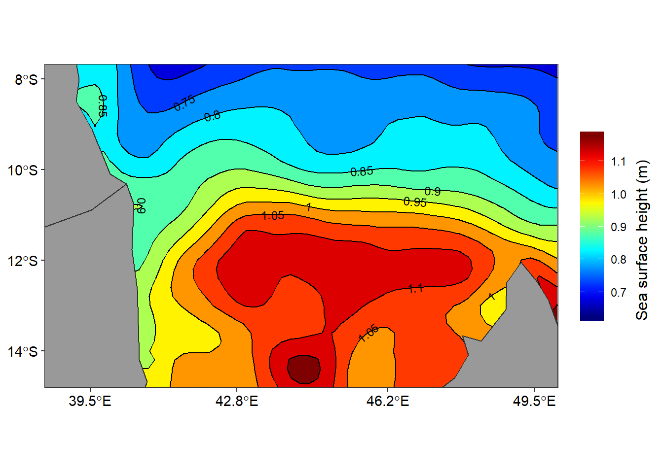
Once the aviso data is tidy and arranged in data frame format, we can use the ggplot2 functions to make maps that show the sea surface height as shown in figure 1 that was created using the lines of code in the chunk below.

ggplot()+
  metR::geom_contour_fill(data = ssh.in, aes(x = lon, y = lat, z = ssh))+
  metR::geom_contour2(data = ssh.in, aes(x = lon, y = lat, z = ssh))+
  metR::geom_text_contour(data = ssh.in, aes(x = lon, y = lat, z = ssh), 
                          parse = TRUE, check_overlap = TRUE, size = 3.2)+
  geom_sf(data = spData::world, fill = "grey60", col = "grey20")+
  coord_sf(xlim = c(39,49.5), ylim = c(-14.5,-8))+
  theme(legend.position = "none")+
  labs(x = NULL, y = NULL)+
  scale_fill_gradientn(name = "ssh (m)",colours = oce::oceColors9A(120), na.value = "white")+
  scale_x_continuous(breaks = seq(39.5, 49.5, length.out = 4) %>%round(1))+
  scale_y_continuous(breaks = seq(-14,-8, 2))+
  guides(fill = guide_colorbar(title = "Sea surface height (m)", 
                               title.position = "right", title.theme = element_text(angle = 90), 
                               barwidth = 1.25, barheight = 10, draw.ulim = 1.2, draw.llim = 0.6))+
  theme_bw()+
  theme(axis.text = element_text(colour = 1, size = 11))

Figure 1: Sea surface height as on 2010-10-22

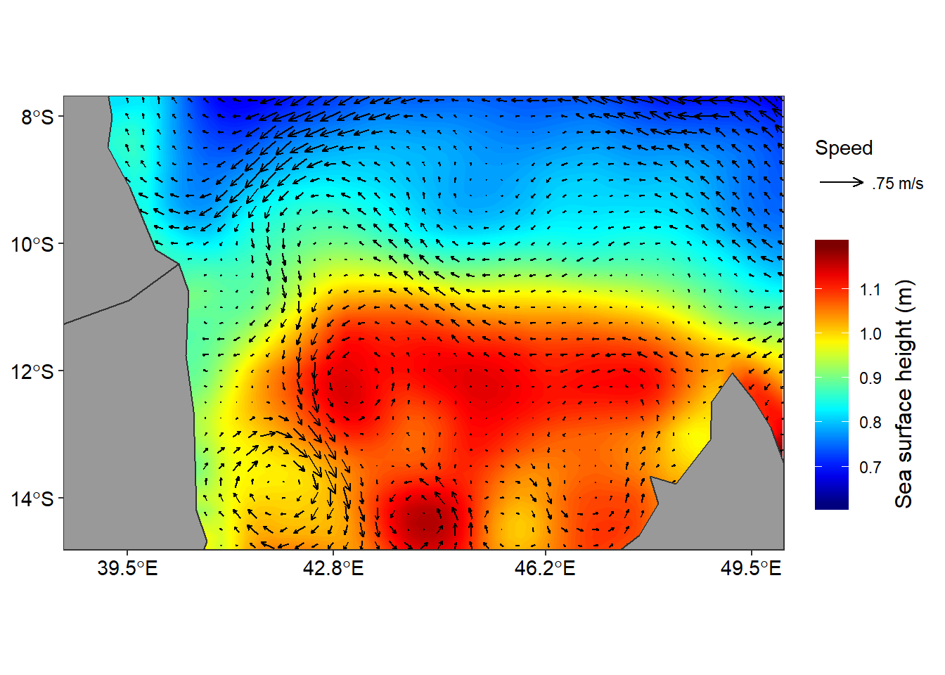
We can also map the geostrophic currents speed and direction on top of the sea surface height as shown in figure 2.

ggplot()+
  metR::geom_contour_fill(data = ssh.in, aes(x = lon, y = lat, z = ssh), bins = 120)+
  metR::geom_vector(data = aviso, aes(x = lon, y = lat, dx = u, dy = v),
                    arrow.angle = 25, arrow.length = .4, arrow.type = "open")+
  metR::scale_mag(max = .75, name = "Speed", labels = ".75 m/s")+
    geom_sf(data = spData::world, fill = "grey60", col = "grey20")+
  coord_sf(xlim = c(39,49.5), ylim = c(-14.5,-8))+
  # theme(legend.position = "none")+
  labs(x = NULL, y = NULL)+
  scale_fill_gradientn(name = "ssh (m)",colours = oce::oceColors9A(120), na.value = "white")+
  scale_x_continuous(breaks = seq(39.5, 49.5, length.out = 4) %>%round(1))+
  scale_y_continuous(breaks = seq(-14,-8, 2))+
  guides(fill = guide_colorbar(title = "Sea surface height (m)", 
                               title.position = "right", title.theme = element_text(angle = 90), 
                               barwidth = 1.25, barheight = 10, draw.ulim = 1.2, draw.llim = 0.6))+
  theme_bw()+
  theme(axis.text = element_text(colour = 1, size = 11))

Figure 2: geostrophic current overalid on the sea surface height

Reference

Mendelssohn, Roy. 2018. Xtractomatic: Accessing Environmental Data from Erd’s Erddap Server. https://CRAN.R-project.org/package=xtractomatic.

Pedersen, Thomas Lin, and David Robinson. 2017. Gganimate: A Grammar of Animated Graphics. http://github.com/thomasp85/gganimate.

Wickham, Hadley. 2016. Ggplot2: Elegant Graphics for Data Analysis. Springer-Verlag New York. http://ggplot2.org.

Wickham, Hadley, Romain François, Lionel Henry, and Kirill Müller. 2018. Dplyr: A Grammar of Data Manipulation. https://CRAN.R-project.org/package=dplyr.