In February 2020, The Institute of Marine Sciences (IMS) in collaboration with Tanzania Fisheries Research Institute (TAFIRI) collected oceanographic variables using CTD in coastal waters of Tanga .The sampled area had three transects from the shallow water below 50 meters deep and cruised to the middle of the Pemba channel. The data collection was completed in three days, each day with one transect. We started sampling with the southmost transect located at Kigombe, followed with the middle and finished with the northern transect located near the Tanga city (Figure 1).
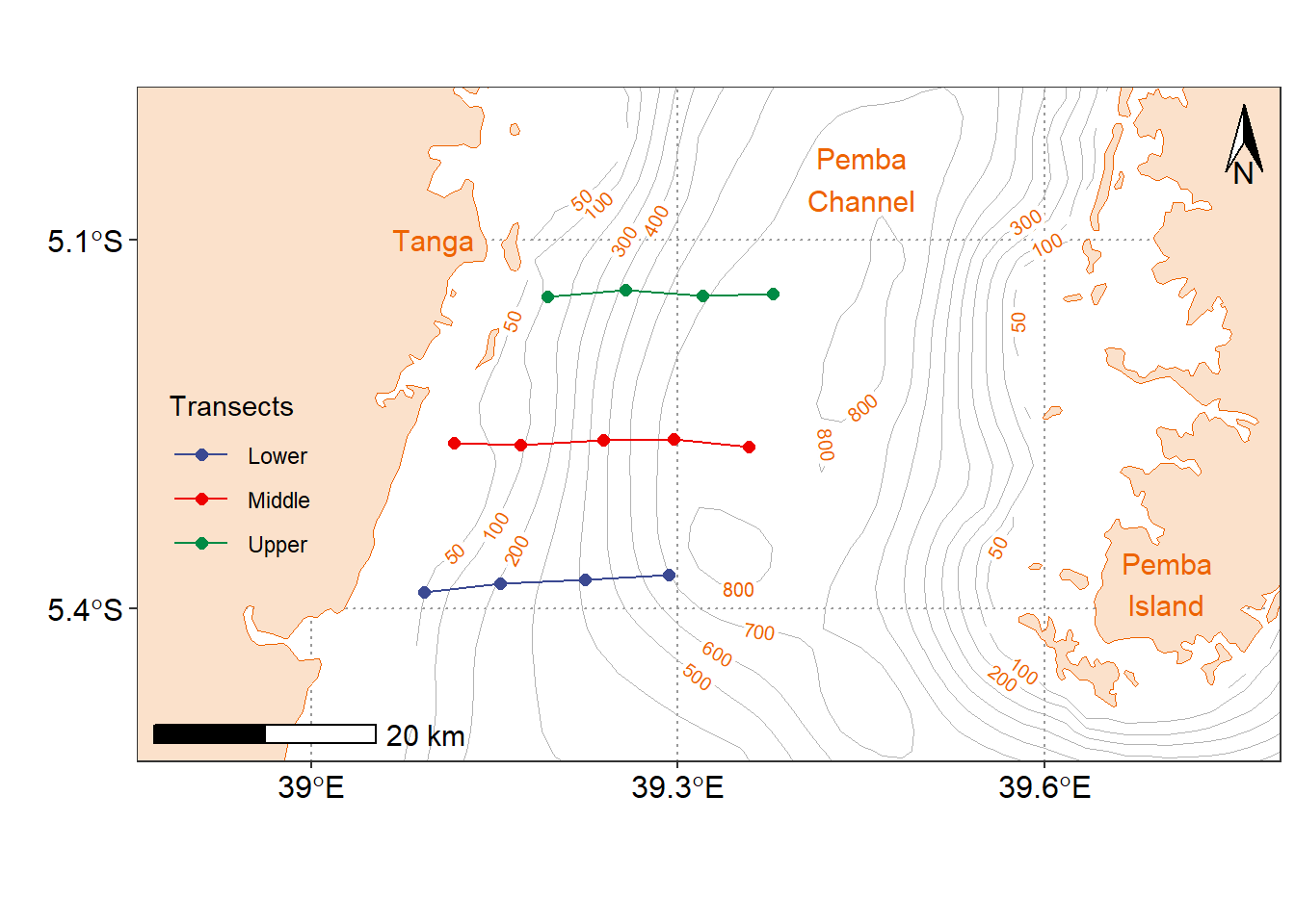
Figure 1: Map of Conductivity-Temperatue-Depth (CTD) cast stations
CTD Profiling
Continuous measurements of temperature, salinity, oxygen and fluorescence were made with a Sea-Bird SBE-9/11Plus CTD package with dual temperature, salinity and oxygen sensors and fluorometer. A CTD cast to depths ranging between 40 and 150 m was conducted at Station during field campaign.
Data Processing
Seabird has a Data Processing software (Seasoft V2) to help massage the data. We processed a bit of data with that and created ‘.cnv’ files and then brought it into R. The function read.ctd.sbe from oce package was used to import Seabird formatted cnv files into R session (Kelley and Richards 2018; Kelley 2015). Once in R session, the CTD cast was further processed. First the the data from downcast were selected and aligned to standard depth of 2 meters interval. Unfortunately our CTD data doesn’t have GPS data. The geographical position data for each cast was integrated into the files. Lastly, the information that describe the people collected the data, the Institute and its address were added as metadata. The post–processing steps was chained in FOR loop to iterate processing of data for each cast as the chunk below highlight;
deepsea.ctd = list()

for (i in 1:length(deepsea.file)) {

  deepsea.ctd[[i]] = read.ctd(deepsea.file[i])%>%
    ctdTrim(method = "downcast")%>%
    ctdDecimate(p = 2)
  deepsea.ctd[[i]]@metadata$scientist = "Semba Masumbuko and Patroba Matiku and Mathew Silas"
  deepsea.ctd[[i]]@metadata$institute = "TAFIRI"
  deepsea.ctd[[i]]@metadata$address = "P.O BOX 9500, Dar es Salaam"
  deepsea.ctd[[i]]@metadata$longitude =ctd.cast.tb$lon[i]
  deepsea.ctd[[i]]@metadata$latitude =ctd.cast.tb$lat[i]
  deepsea.ctd[[i]][["oxygen"]] = deepsea.ctd[[i]][["oxygen2"]]


}
Results
Figure 2 and 3 show a typical CTD profiles. While 2 use unesco to get the older seawater formulation, a figure 3used the newer gsw seawater formulation. These figure 3 show partial temperature and salinity change with water depth. As the depth increases (moving down on the vertical axis), temperature (in red) increases, until a maximum is reached at a depth of 50 meters.
Salinity, shown in green, increases rapidly with depth, until about 60 meters deep, where it increases only very slowly to about 35.3 absolute salinity ([g/kg]). Note that the differences being measured here are very small 0.1 degrees C and 0.01 ppt (Figure 3.
deepsea.ctd[[8]] %>%
  oce::plot(eos = "unesco",
  useSmoothScatter = FALSE, grid = F,
  showHemi = FALSE,
  drawIsobaths = TRUE)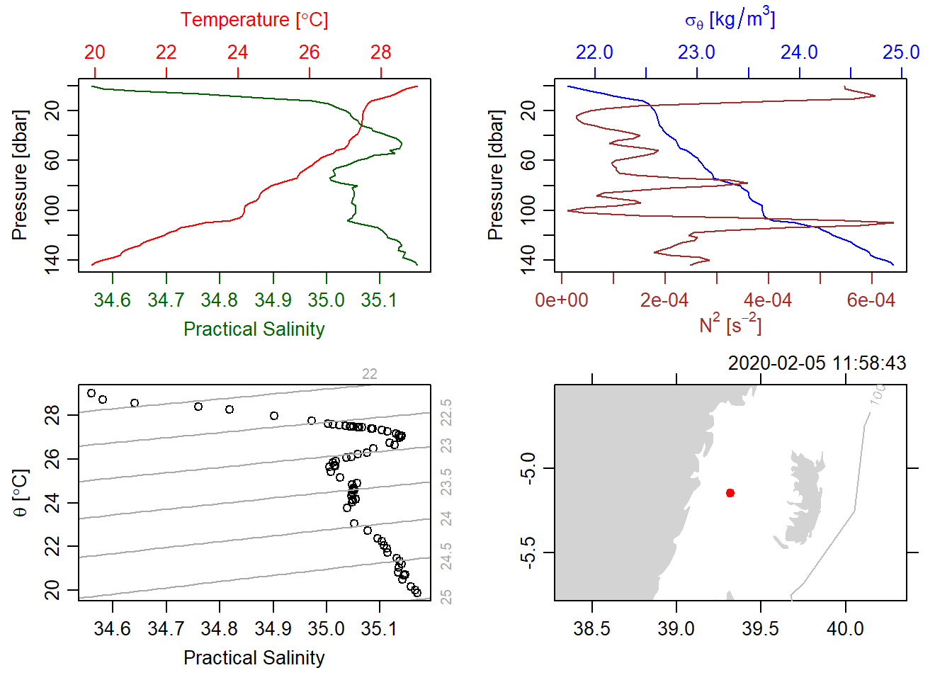
Figure 2: A typical CTD Plots showing profiles of salinity and temperature (topleft), profiles of density and the square of buoyancy frequency (topright), a TS diagram (bottomleft) and a coastline diagram indicating the station location (bottomright) using the unesco equation of state.
deepsea.ctd[[8]] %>%
  oce::plot(eos = "gsw",
  useSmoothScatter = FALSE, grid = F,
  showHemi = FALSE,
  drawIsobaths = TRUE)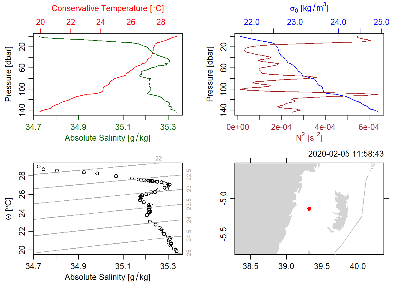
Figure 3: A typical CTD Plots showing profiles of salinity and temperature (topleft), profiles of density and the square of buoyancy frequency (topright), a TS diagram (bottomleft) and a coastline diagram indicating the station location (bottomright) using the gsw equation of state.
Cross–section
Then, the multiple CTD casts were stitched together to form a section. Section requires the multiple CTD cast organized in a list file. This was done already in section ??. The function as.section from oce package was used to create a section file.
all.transects = deepsea.ctd %>% as.section()## Warning in as.section(.): estimated waterDepth as max(pressure) for CTDs
## numbered 1:10subset the transect of interest from the section. For our case, we can simply extract a transect using the indices. Once transect is extracted from the section was used make a basic contour plot (Figure 4 and image plot (Figure 5.
all.transects %>%
  subset(indices = 7:10)%>%
  plot(which = c("temperature", "oxygen", "fluorescence", "salinity"),
       ztype = "contour", xtype = "longitude", eos = "gsw")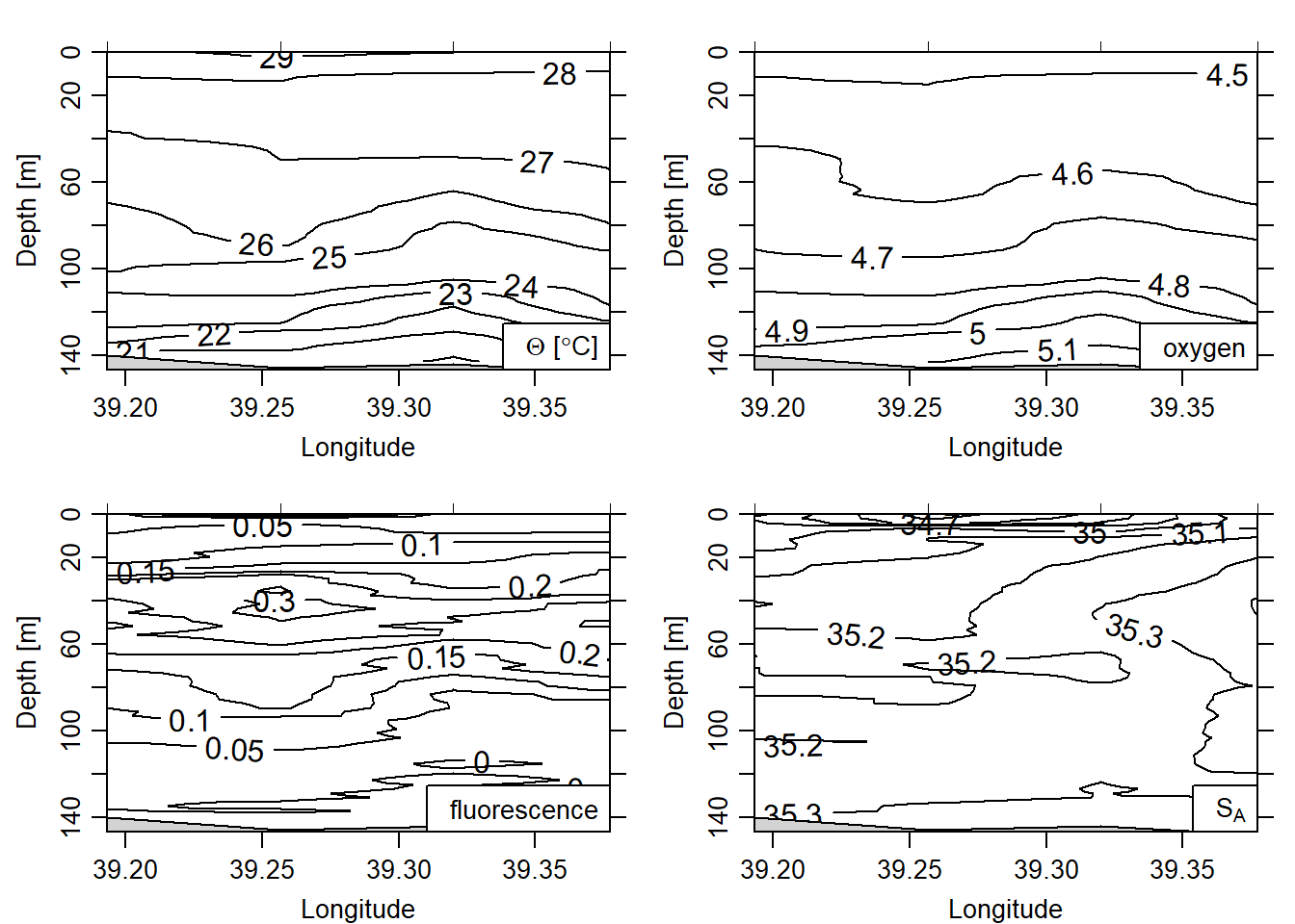
Figure 4: Contour plot
all.transects %>%
  subset(indices = 7:10)%>%
  plot(which = c("temperature", "oxygen", "fluorescence", "salinity"),
       ztype = "image", xtype = "longitude", filledContours=FALSE, eos = "gsw")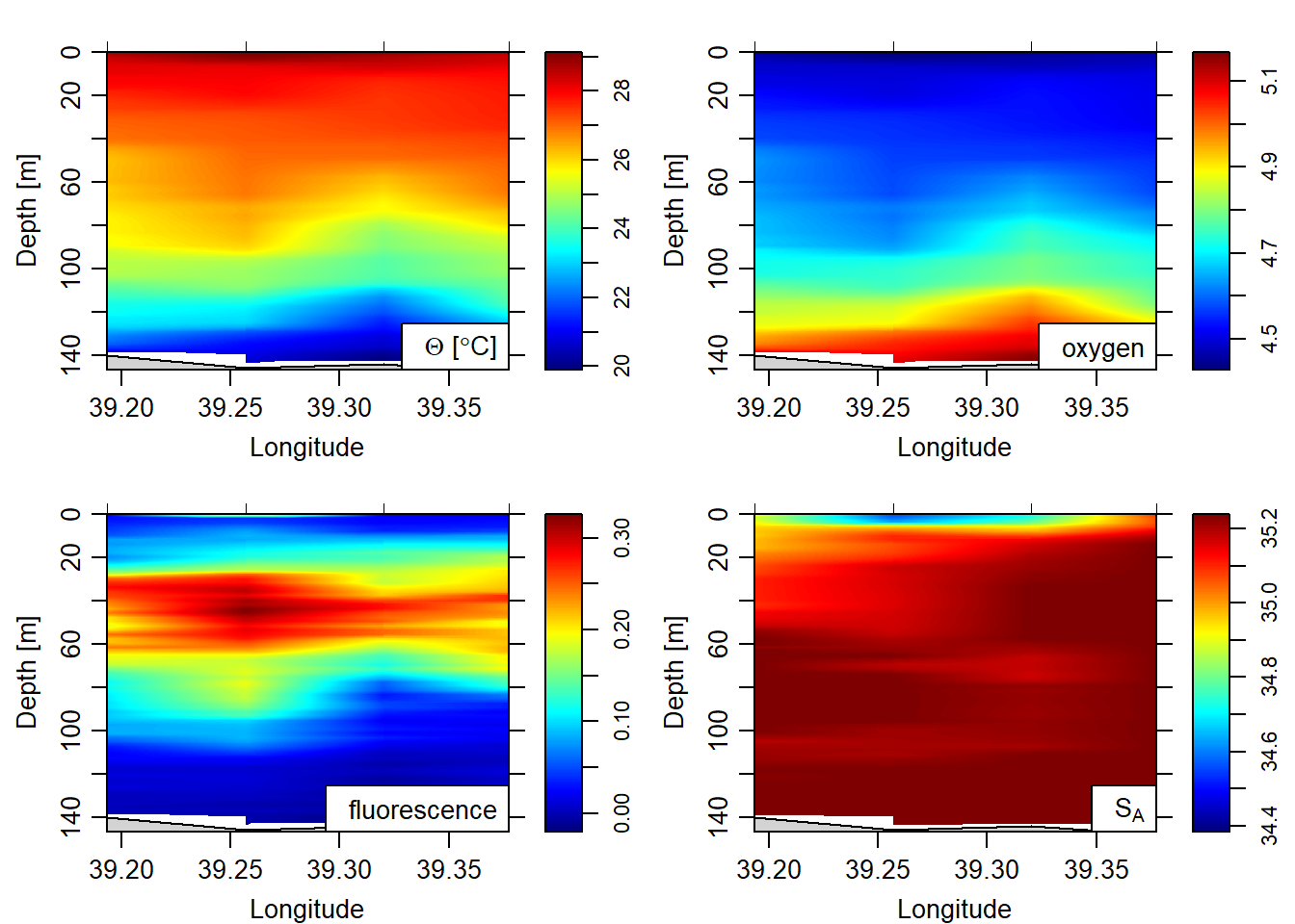
Figure 5: image plot
Fluorescence comes from the fluorometer, which measures the quantity of primary producers in the water column. You can see in figure 5 that mid-water peaks phytoplankton at the thermocline (where the there is a rapid temperature change). This probably reflects the zone of mixing between deeper nutrient rich waters and shallower brighter waters (but nutrient poor).
Reference
Kelley, Dan. 2015. Ocedata: Oceanographic Datasets for Oce. https://CRAN.R-project.org/package=ocedata.
Kelley, Dan, and Clark Richards. 2018. Oce: Analysis of Oceanographic Data. https://CRAN.R-project.org/package=oce.