Any quantitative value measured over regular time intervals makes a Time Series. Time-series analysis aims to investigate the temporal behavior of a variable \(X_{t}\). Examples include the investigation of long-term records of sea surface temperature, sea-level fluctuations, millennium-scale variations in the atmosphere-ocean system, the eff ect of the El-Niño/Southern Oscillation on tropical rainfall and sedimentation (Trauth 2015). R has extensive facilities for analyzing time series data. These packages provides various tools with which to detect these temporal patterns. Understanding the underlying processes that produced the observed data allows us to predict future values of the variable.
This post describes how to create time series objects, decompose the time series into seasonal, trend and error components. We use the lubridate(Grolemund and Wickham 2011), tidyverse Wickham (2017)] package to tidy and process the date and data; ts and forecast(Hyndman et al. 2018) packages for creating and manipulating time series objects and oce(Kelley and Richards 2018) and ggplot2(Wickham 2016) packages to visualize the outputs of the time series.
require(tidyverse)
require(lubridate)
require(oce)
require(lubridate)
require(forecast)
Dataset
In this post we use the daily sea surface temperature collected near Chumbe Island in Unguja with a data logger for a period of 21 years —from January 01, 1997 to December 31, 2017. The data is in excel, therefore, we import the dataset into the workspace with the readxl::read_excel() function.
all = readxl::read_excel("E:/Data Manipulation/Temperature data/processing/Chumbe_SST_Temperature 1997-30Nov2017_IMS_Muhando.xlsx")The data comes in wide format—multiple columns—each column represent a year. Therefore, this dataset was converted from multiple columns format —wide format into a long format.The chunk below simply highlight the transformation steps.
## change from wide form to long form with gather function

all = all %>% gather(key = "year", value = "sst", 2:22)
We notice that the February month has been treated with 29 days for all the years. Some years are short with only 28 days. Table 1 highlight the wrongly entered temperature values for the 29th February for years which end on the 28th. Therefore all these values must be trimmed off.
index =which(all$sst> 500)

all %>% slice(index) %>% separate(day, c("Year", "Month", "Day"), sep = "-") %>% unite(Date, c("Day", "Month", "year"), sep = "-") %>% select(-Year) %>% kableExtra::kable(format = "html", col.names = c("Date", "Temperature"), caption = "Wrongly entered temperature values") %>%
kableExtra::column_spec(column = 1:2, width = "3 cm")| Date | Temperature |
|---|---|
| 29-02-1997 | 1000 |
| 29-02-1998 | 1000 |
| 29-02-1999 | 1000 |
| 29-02-2001 | 1000 |
| 29-02-2002 | 1000 |
| 29-02-2003 | 1000 |
| 29-02-2005 | 1000 |
| 29-02-2006 | 1000 |
| 29-02-2007 | 1000 |
| 29-02-2009 | 1000 |
| 29-02-2010 | 1000 |
| 29-02-2011 | 1000 |
| 29-02-2013 | 1000 |
| 29-02-2014 | 1000 |
| 29-02-2015 | 1000 |
| 29-02-2017 | 1000 |
The chunk below highlight code of lines that I used to clean the dataset by removing the wrongly entered temperature values for the day 29 for years ending on the 28th.
all.tb = all %>%
  filter(is.na(sst)) %>%
  bind_rows(all %>%
              filter(sst > 15 & sst < 40)) %>%
  separate(day, c("mwaka", "month", "siku"), sep = "-") %>%
  separate(siku, c("siku", "muda"), sep = " ") %>%
  mutate(date = make_date(year, month, siku)) %>%
  arrange(date) %>%
  select(date, sst)
Figure 1 show that some years the temperature values are missing. For us to use these data in time series it must be complete, with each day with a values.
all.tb = all.tb %>% mutate(year = year(date), day.year = yday(date))

ggplot(data = all.tb, aes(y = day.year, x = year))+
  geom_raster(aes(fill = sst), interpolate = F)+
  geom_contour(aes(z = sst), col = "black", bins = 3 )+
  theme(plot.background = element_blank(),
        legend.position = "bottom",
        panel.border = element_blank(),
        axis.text = element_text(colour = "black", size = 11),
        axis.title = element_text(colour = 1, size = 12),
        legend.key.width = unit(30, "mm"),
        legend.key.height = unit(4, "mm"),
        legend.title = element_text(size = 12),
        legend.text = element_text(size = 11))+
  scale_x_continuous(breaks = seq(1997,2017,2), position = "top") +
  scale_y_reverse(breaks = seq(15,370,30)
                  # labels = month(seq(dmy(010119), dmy(021219),
                  #                    by = "month"), label = T, abbr = F)
                  )+
  scale_fill_gradientn(colours = oceColorsJet(210),
                       na.value = NA,
                       breaks =seq(24.5,31,1))+
  guides(fill = guide_colorbar(title = expression (Temperature~(degree~C)),
                               title.position = "top", title.hjust = 0.5,
                               title.vjust = 0.25,
                               label.vjust = 1, raster = TRUE, frame.colour = NULL,
                               ticks.colour = 1, reverse = FALSE)) +
  labs(x = "", y = "Number of days in a Year")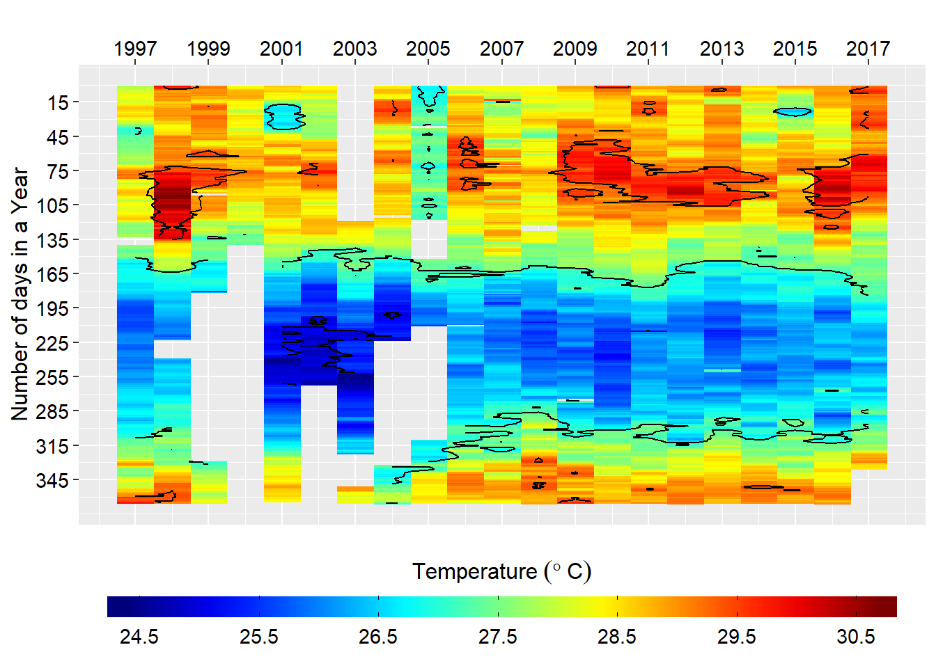
Figure 1: Heatmaps of daily sea surface temperature
As we have in figure 1 there gaps in our dataset—with some years missing data for more than six year period. Since the time series dont like the missing data, we will fill the missing data with an interpolation. We use the oce::interpBarnes() function to predict the missing temperature values in our dataset. The chunk below highlight the key procedure of using oce::interpBarnes() function. Figure 2 show the origin temperature values and the interpolated ones. The codes used to create this figures are highlighted in the chunk below.
## define the total number of days in a year
days = 1:366
#define the total number of years as indicated by the data
years = 1997:2017


par(mfrow = c(2,1))

## make a matrix using the origin temperature values
all.mat = matrix(all.tb$sst, nrow = length(days))
## plot the matrix
imagep(y = years, x = days, z = all.mat, filledContour = F, ylim = c(2017,1997),zlab = expression(Temperature~(degree *C)), xlab = "Day")
contour(y = years, x = days, z = all.mat, add = TRUE, col = 1, nlevels = 3)

## interpolate the missing values
interpolated.temperature = interpBarnes(x = all.tb$day.year, y = all.tb$year, z = all.tb$sst, xgl = 366, ygl = 21)

## plot the interpolated values
imagep(x = interpolated.temperature$xg, y = interpolated.temperature$yg, z = interpolated.temperature$zg, filledContour = F, ylim = c(2017,1997),zlab = expression(Temperature~(degree *C)), xlim = c(1,360), xlab = "Day")
contour(x = interpolated.temperature$xg, y = interpolated.temperature$yg, z = interpolated.temperature$zg, col = 1, nlevels = 4,add = TRUE)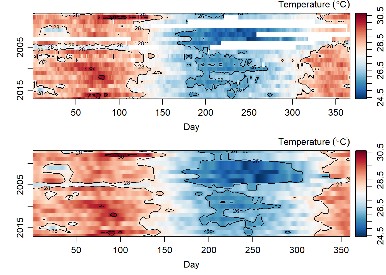
Figure 2: Temperature values for origin data (top panel) and interpolated values (bottom panel)
As we have observed, time series analysis hate missing values (Figure 2) and since we managed to fill the missing values with an interpolation technique (Figure 2), we can now work with the function in time series. Unfortunate the matrix temperature interpolated data is longer than the period of the data duration. Therefore, we convert it data frame and then remove again a day in years with only days in February. The chunk below contains the codes that was used for cleaning and transformation of the interpolated dataset.
## extracted the matrix of interpolated values
interpolated.sst.mat = interpolated.temperature$zg
## check the dimension if is 366 days and 21 years (1997:2017)
dim(interpolated.sst.mat)
[1] 366 21## tranform the matrix into the tabular form and combine the interpolated values with the raw
interpolated.sst.tb = interpolated.sst.mat %>%
as.tibble() %>%
gather(key = "year", value = "sst",1:21) %>%
select(-year, sst.interp = sst)%>%
bind_cols(all)
## make an index of short years of 28 days in february that appear with 29 days
index = which(all$sst ==1000)
## check if the wrong days exist
interpolated.sst.tb %>% slice(index)# A tibble: 16 x 4
sst.interp day year sst
<dbl> <dttm> <chr> <dbl>
1 27.7 2016-02-29 00:00:00 1997 1000
2 29.1 2016-02-29 00:00:00 1998 1000
3 29.5 2016-02-29 00:00:00 1999 1000
4 28.6 2016-02-29 00:00:00 2001 1000
5 28.6 2016-02-29 00:00:00 2002 1000
6 28.8 2016-02-29 00:00:00 2003 1000
7 27.4 2016-02-29 00:00:00 2005 1000
8 29.4 2016-02-29 00:00:00 2006 1000
9 29.0 2016-02-29 00:00:00 2007 1000
10 29.8 2016-02-29 00:00:00 2009 1000
11 29.3 2016-02-29 00:00:00 2010 1000
12 29.0 2016-02-29 00:00:00 2011 1000
13 28.8 2016-02-29 00:00:00 2013 1000
14 28.7 2016-02-29 00:00:00 2014 1000
15 28.8 2016-02-29 00:00:00 2015 1000
16 29.3 2016-02-29 00:00:00 2017 1000 ## trim off the dataset all short years with the wrong 29th February
interpolated.sst.tb = interpolated.sst.tb %>% slice(-index)
## now the data is clean we can sequeance the number of days with
interpolated.sst.tb = interpolated.sst.tb %>%
mutate(date = seq(dmy(010197), dmy(311217), by = "day")) %>%
select(date, sst.interp, sst.original =sst)Creating a time series
The ts() function convert a numeric vector into an R time series object. The format is ts(vector, start=, end=, frequency=) where start and end are the times of the first and last observation and frequency is the number of observations per unit time (1=annual, 4=quartely, 12=monthly,365.24=daily, etc.). Our dataset contain daily sea surface temperature observations from 1997-01-01 to 2017-12-31. The time series for this object was created with the line code in the chunk below
temperature.ts = ts(data = interpolated.sst.tb$sst.interp,
                    start = c(1997,1),
                    frequency = 365.24)

temperature.ts %>% plot(ylab = expression(Temperature~(degree*C)))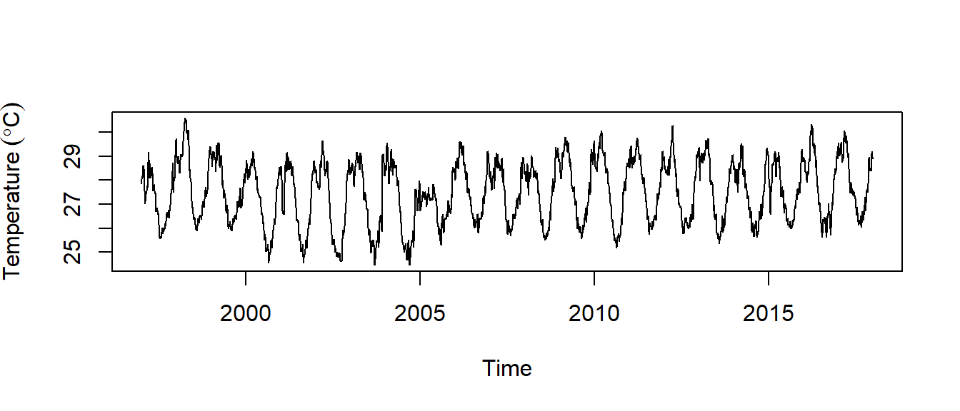
Figure 3: Time seris of sea surface temperture
We can see from figure 3 that there seems to be seasonal variation in the daily temperature at Chumbe—there is a peak every northeast monsoon season, and a trough every southeast monsoon. Again, it seems that this time series could probably be described using an additive model, as the seasonal fluctuations are roughly constant in size over time and do not seem to depend on the level of the time series, and the random fluctuations also seem to be roughly constant in size over time
We notice in figure 3 that the temperature declined gradually from 1997 and reached its lowest in 2006 and then raised in 2007 and has been oscilating ever since. We can split the two epoch with the window() function and plot the two epochs shown in figure 4. The code for spliting the time series and make plots shown in figure 4 is highlighted in the chunk below.
par(mfrow = c(1,2))
epoch1 = window(x = temperature.ts, start = c(1997,1), end = c(2005,12))
epoch1 %>% plot(main = "Before January 2006")

epoch2 = window(x = temperature.ts, start = c(2007,1), end = c(2017,12))
epoch2 %>% plot(main = "After December 2006")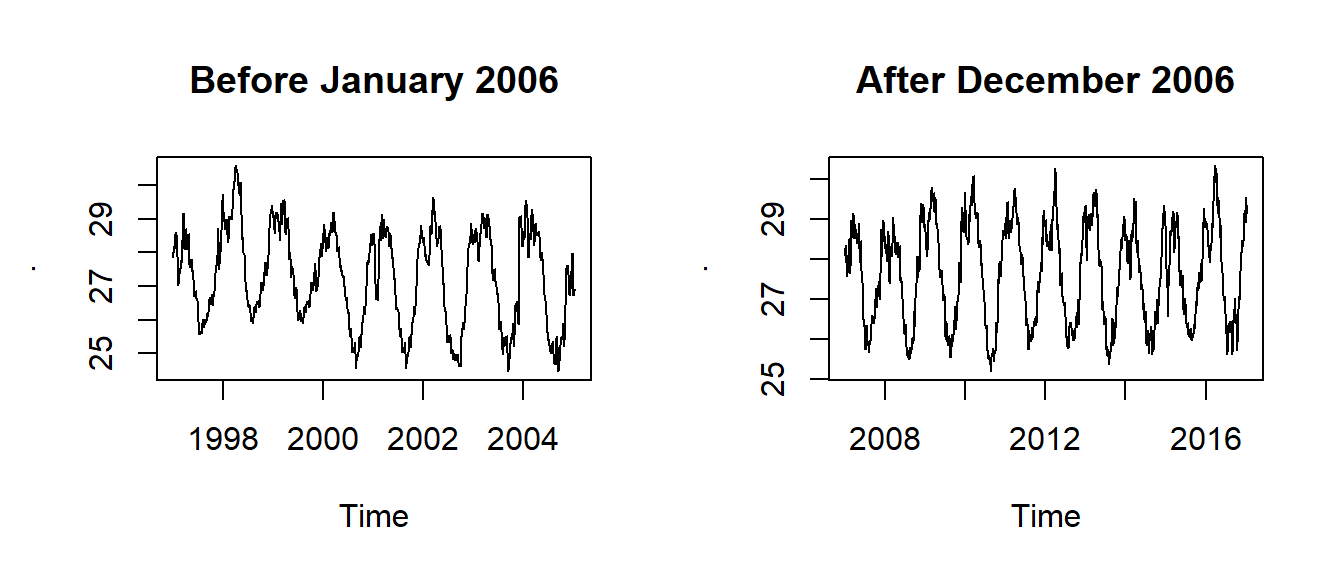
Figure 4: Time series before 2006 (top panel) and after 2006 (bottom panel)
Decomposing Time Series
Decomposing a time series means separating it into its constituent components, which are usually a trend component and an irregular component, and if it is a seasonal time series, a seasonal component.
Decomposing Seasonal Data
A seasonal time series consists of a trend component, a seasonal component and an irregular component. Decomposing the time series means separating the time series into these three components: that is, estimating these three components.
To estimate the trend component and seasonal component of a seasonal time series that can be described using an additive model, we can use the decompose() function in R. This function estimates the trend, seasonal, and irregular components of a time series that can be described using an additive model.
The function decompose() returns a list object as its result, where the estimates of the seasonal, trend and irregular component are stored in named elements of that list objects, called seasonal, trend, and random, respectively.
For example, given the daily temperature in Chumbe Island is seasonal with a maximum during the northeast season and minimum in southeast period, and can probably be described using an additive model since the seasonal and random fluctuations seem to be roughly constant in size over time. The chunk below highlight the codes that we can type to estimate the trend, seasonal and irregular components of this time series. The decompose() and forecast::stl() splits the time series into these time series components;
temperature.components = decompose(temperature.ts)The estimated values of the seasonal, trend and irregular components are now stored in variables temperature.components$seasonal, temperature.components$trend and temperature.components$random. For example, we can print out the estimated values of the seasonal component by typing:
temperature.components$seasonalThe estimated seasonal factors are given for the days. The positive (largest seasonal factor) day 1 to 151 which coincide with the NE season and the negative value (small seasonal factor) is from day 152 to day 320, which appears on SE season. These seasonal factor are the same each year from 1997 to 2017, indicating that there seems to be a peak in temperature in NE and a trough in temperature in SE each year. Figure 5 show the estimated trend, seasonal, and irregular components of the time series created with the line of code in the chunk here:
temperature.components %>% plot()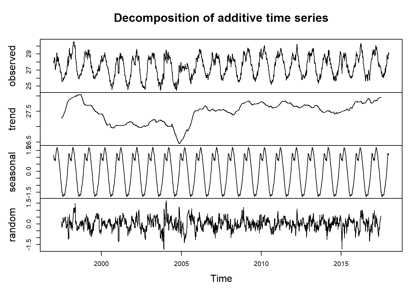
Figure 5: Decomposition of additive time series
Figure 5 show the original time series (top), the estimated trend component (second from top), the seasonal third from top), and the irregular component (bottom). We see that the estimated trend component shows a small decrease from about 28 in 1998 to about 26.5 in 2006, followed by a steady increase from then on to about 28 in 2017.
Seasonally Adjusting
If you have a seasonal time series that can be described using an additive model, you can seasonally adjust the time series by estimating the seasonal component, and subtracting the estimated seasonal component from the original time series. We can do this using the estimate of the seasonal component calculated by the decompose() function.
For example, to seasonally adjust the time series of the daily temperature in Chumbe Island, we can estimate the seasonal component using “decompose()”, and then subtract the seasonal component from the original time series:
par(mfrow = c(2,1))
par(mar = c(2.5,2.5,0,0))

temperature.ts %>% plot(labels = FALSE, xlab = "")
# draw an axis on the left
Axis(side=2, labels=TRUE, las = 2)


temperature.ts.adjusted = temperature.ts -temperature.components$seasonal
temperature.ts.adjusted %>% plot(xlab = "")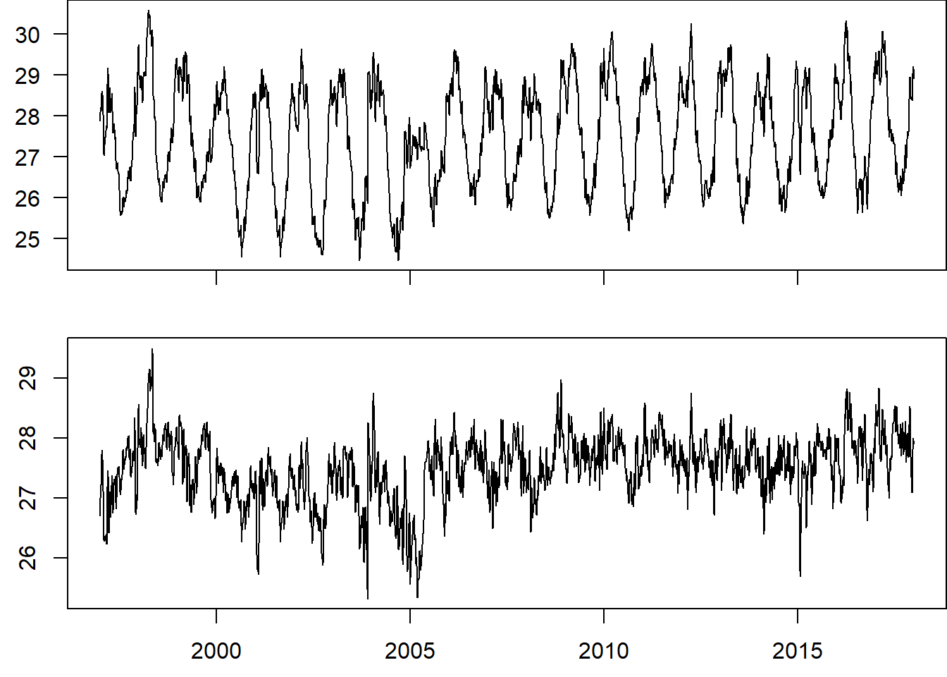
Figure 6: Time series of sea surface temperature before removing the seasonal variation (top pane) and after the seasonality removed (bottom panel)
You can see from figure 6 the seasonal variation has been removed from the seasonally adjusted time series. The seasonally adjusted time series now just contains the trend component and an irregular component.
References
Grolemund, Garrett, and Hadley Wickham. 2011. “Dates and Times Made Easy with lubridate.” Journal of Statistical Software 40 (3): 1–25. http://www.jstatsoft.org/v40/i03/.
Hyndman, Rob J, George Athanasopoulos, Christoph Bergmeir, Gabriel Caceres, Leanne Chhay, Mitchell O’Hara-Wild, Fotios Petropoulos, Slava Razbash, Earo Wang, and Farah Yasmeen. 2018. “Forecast: Forecasting Functions for Time Series and Linear Models.”
Kelley, Dan, and Clark Richards. 2018. Oce: Analysis of Oceanographic Data. https://CRAN.R-project.org/package=oce.
Trauth, Martin. 2015. MATLAB® Recipes for Earth Sciences. Book. 4th ed. 2015. Berlin, Heidelberg: Berlin, Heidelberg : Springer Berlin Heidelberg : Imprint Springer.
Wickham, Hadley. 2016. Ggplot2: Elegant Graphics for Data Analysis. Springer-Verlag New York. http://ggplot2.org.
———. 2017. Tidyverse: Easily Install and Load the ’Tidyverse’. https://CRAN.R-project.org/package=tidyverse.