In the previous post, we explore the power of oce package in mapping oceanographic data. In this post we will continue that theme and dive to process topographic data and map the bathymetry. We will grab ETOPO1 dataset— a 1 arc-minute global relief model that integrates land topography and ocean bathymetry. We will process the data and then use different ways to visualize the bathymetric information. There is no much statistics or modelling in this post, but the post focus on letting you know how to process the ascii (.asc) file and transform it to a format that functions in oce package understand (Kelley and Richards 2018). We need functions from some packages, hence to use their functions we need to load these packages into our workspace.
require(tidyverse)
require(oce)
require(ocedata)
The ETOPO1 dataset downloaded as an ascii file and used the function read.asciigrid() to read and import it from the working directory in my local machine into R’s workspace (R Core Team 2018). The imported files was assigned name as etopo
etopo = sp::read.asciigrid("./Tanzania_etopo1/tanz1_-3432.asc")The asciigrid() function produce the SpatialGridDataFrame object. Although this SpatialGridDataFrame object fits for plotting using base R graphic, its incompatible with oce plotting. The mapping function of oce likemapImage() and mapContour() require the z–variable to be in grid or matrix class. We tranform this class into data frame rename the variables with meaningful names. The data frame now has three variables—longitude, latitude and topographic values—treated as elevation though does store the elevation and bathymetry.
etopo.df = etopo %>%
  as.tibble() %>%
  select(lon = 2, lat = 3, elevation = 1 )
Our file now is in the xyz format and still we can not use the function in oce package to map the bathymetry and contour of the oceans. To make these dataset work in oce, we have to transform it further to matrix. We can achieve this by knowing the number of rows and columns contained in the dataset. However, if you do know them, then extract the longitude and latitude from the data frame we created above and spite out only the unique values. The chunk below show the procedure
lon = etopo.df$lon %>% unique()
lat = etopo.df$lat %>% unique()
elevation = etopo.df$elevation

# length(lon); length(lat); length(elevation) # uncomment to pring the values
We notice that the number of columns are 781 and of rows are 841. We use this information to make a matrix as shown in the chunk below
etopo.mat = matrix(data = elevation,
                   nrow = length(lat),
                   ncol = length(lon),
                   byrow = TRUE)
After exploring, I notice that the matrix I created does not match the length of longitude na latitude. The function t() was used to transpose th matrix. Then create the file that contains only the bathymetric value. This was done by assigning all land values with an NA. The chunk here hgighlight the main steps
etopo.mat = etopo.mat %>% t()
etopo.ocean = etopo.mat
    etopo.ocean[etopo.ocean > 0] = NA
The ocedata package comes with world boundary shapefiles (Kelley 2015). We need these dataset as basemaps—that provide background details for the maps we are going to make. We load these basemaps into the workspace as shown in the chunk below.
data("coastlineWorld")
data("coastlineWorldMedium")
data("coastlineWorldFine")
We have all the dataset, the basemaps and the gridded bathymetry data in the format that oce understand. The figure 1 was created using lines of codes highlighted in the chunk below.
## regional map
cm <- colormap(name="gmt_globe")

lonlim = c(38.5,43)
latlim = c(-6,-4)
zlim = c(-5000,0)

par(mar = c(2,2,1,2))
drawPalette(zlim = zlim, at = seq(-5000,0,1000),
            labels = seq(5000,0,-1000), pos = 4, colormap = cm)
mapPlot(coastlineWorld,
        longitudelim = lonlim,
        latitudelim = latlim,
        projection = "+proj=mill",
        col = "lightgray",
        grid = c(0.75,0.75), clip = TRUE)
mapImage(longitude = lon, latitude = lat, z = etopo.ocean, colormap = cm, zclip = TRUE)
mapContour(longitude = lon, latitude = lat, z = etopo.ocean,
           levels = seq(-5000,0,1000), col = "black", lty = 1, lwd = 1)
mapPolygon(coastlineWorldFine, col = "lightgray", border = "black")
mapGrid(dlongitude = 0.75, dlatitude = 0.75, lty = 3, lwd = .5)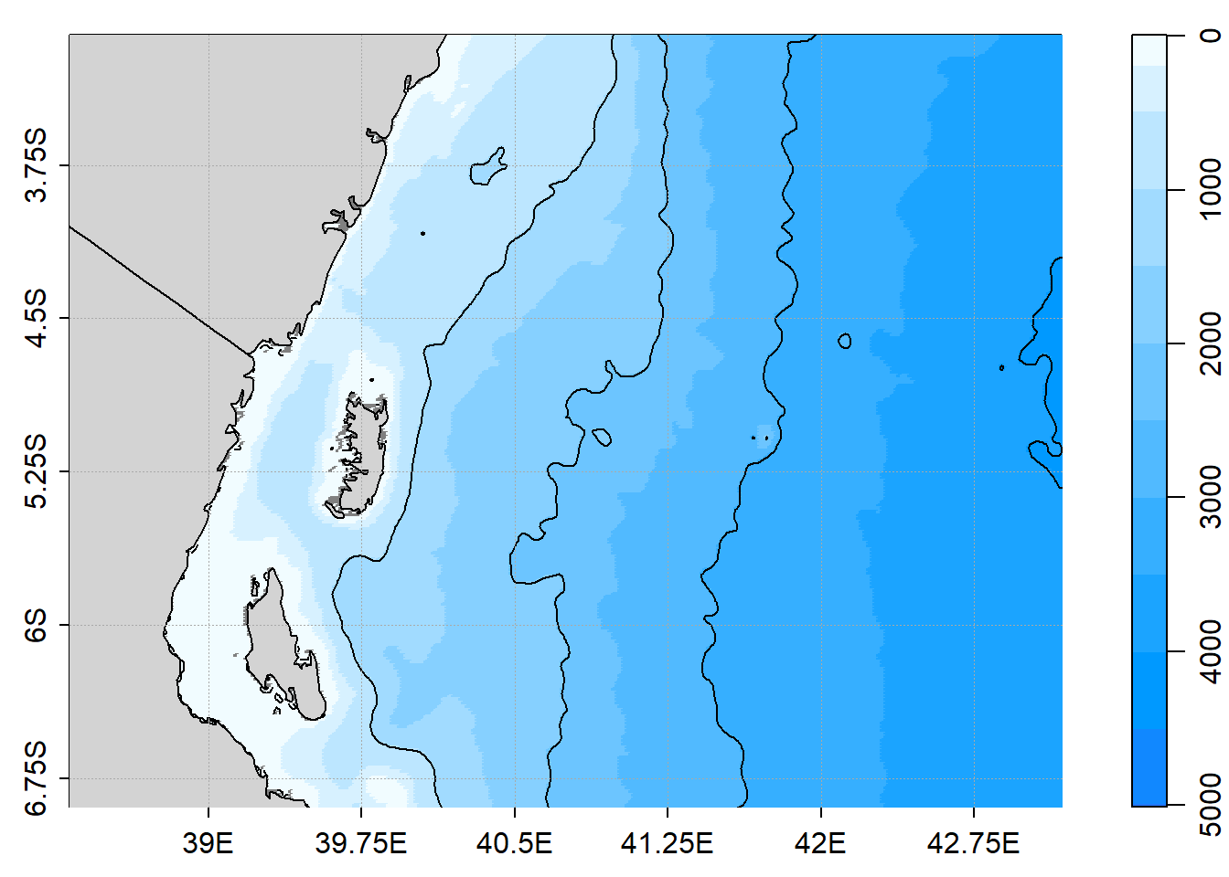
Figure 1: Figure 1
I then defined the geographical limits—longitude and latitude bounds to make a plot of pemba channel shown in figure 2. The lines of codes to make this figure are shown in the chunk below.
## local Pemba
cm <- colormap(name="gmt_globe")

lonlim = c(39,40)
latlim = c(-5.5,-4.5)
zlim = c(-2000,0)

par(mar = c(2,2,1,2))
drawPalette(zlim = zlim, at = seq(-2000,0,500),
            labels = seq(2000,0,-500), pos = 4, col = oce.colorsGebco(120))
mapPlot(coastlineWorldFine,
        longitudelim = lonlim,
        latitudelim = latlim,
        projection = "+proj=mill",
        col = "lightgray",
        grid = c(0.3,0.25), clip = TRUE)
mapImage(longitude = lon, latitude = lat, z = etopo.ocean,  zlim = c(-2000,0),
         zclip = TRUE,filledContour = FALSE, gridder = "interp", col = oceColorsGebco(120))
mapContour(longitude = lon, latitude = lat, z = etopo.ocean,levels = seq(-200,0,50),
            col = "lightgrey", lty = 1, lwd = 1)
mapContour(longitude = lon, latitude = lat, z = etopo.ocean,levels = seq(-2000,-300,100),
            col = "black", lty = 1, lwd = 1)
mapPolygon(coastlineWorldFine, col = "lightgray", border = "black")
mapGrid(dlongitude = 0.3, dlatitude = 0.25, lty = 3, lwd = .5)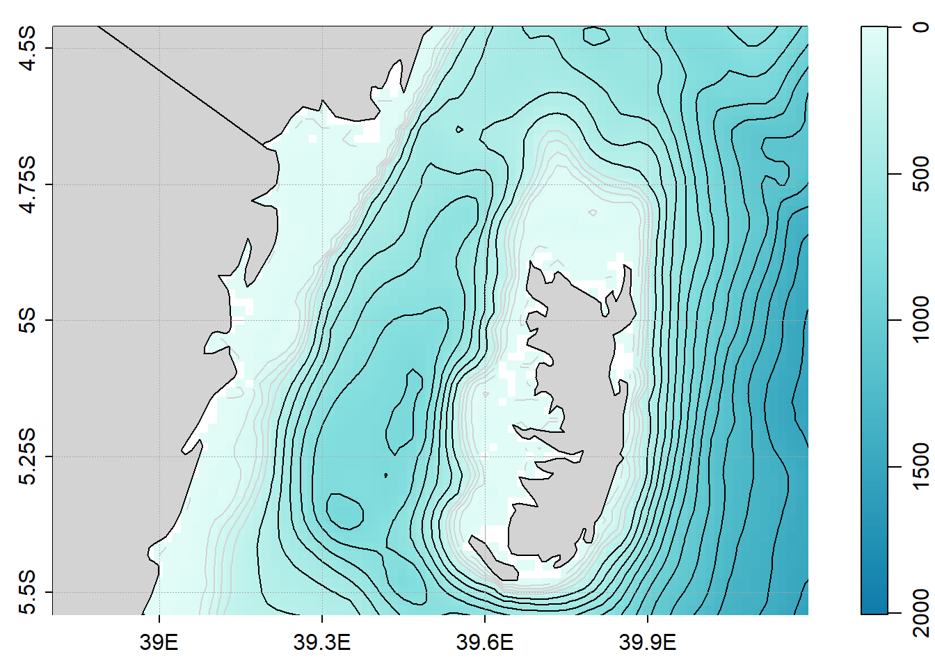
Figure 2: Bathymetric map of Pemba channel. The black lines are contour interval of 100 meters and the grey line are contour interval of 50 meters.
Further down in around latitude 11oS is the pinacle where the south equatorial current splits and form the northward flowing—the East African Coastal Current and southward flowing—the Mozambique current. I was interested to visualize the bottom topography within this area. I defined the geographical extent to map the bathymetry in this region. The codes to make map showin in Figure 3 are in this chunk.
## local Mtwara
cm <- colormap(name="gmt_globe")

lonlim = c(40,42)
latlim = c(-11.0,-10.0)
zlim = c(-3500,0)

par(mar = c(2,2,1,2))
drawPalette(zlim = zlim, at = seq(-3500,0,500),
            labels = seq(3500,0,-500), pos = 4, col = oce.colorsGebco(120))
mapPlot(coastlineWorldFine,
        longitudelim = lonlim,
        latitudelim = latlim,
        projection = "+proj=mill",
        col = "lightgray",
        grid = c(0.5,0.5), clip = TRUE)
mapImage(longitude = lon, latitude = lat, z = etopo.ocean,  zlim = c(-3600,0),
         zclip = TRUE,filledContour = FALSE, gridder = "interp", col = oceColorsGebco(120))
mapContour(longitude = lon, latitude = lat, z = etopo.ocean,levels = seq(-3500,-600,200),
            col = "grey80", lty = 1, lwd = 0.25)
mapContour(longitude = lon, latitude = lat, z = etopo.ocean,levels = seq(-3500,-500,500),
            col = "black", lty = 1, lwd = 1)
mapPolygon(coastlineWorldFine, col = "lightgray", border = "black")
mapGrid(dlongitude = 0.5, dlatitude = 0.5, lty = 3, lwd = .5)
mapScalebar(length = 20)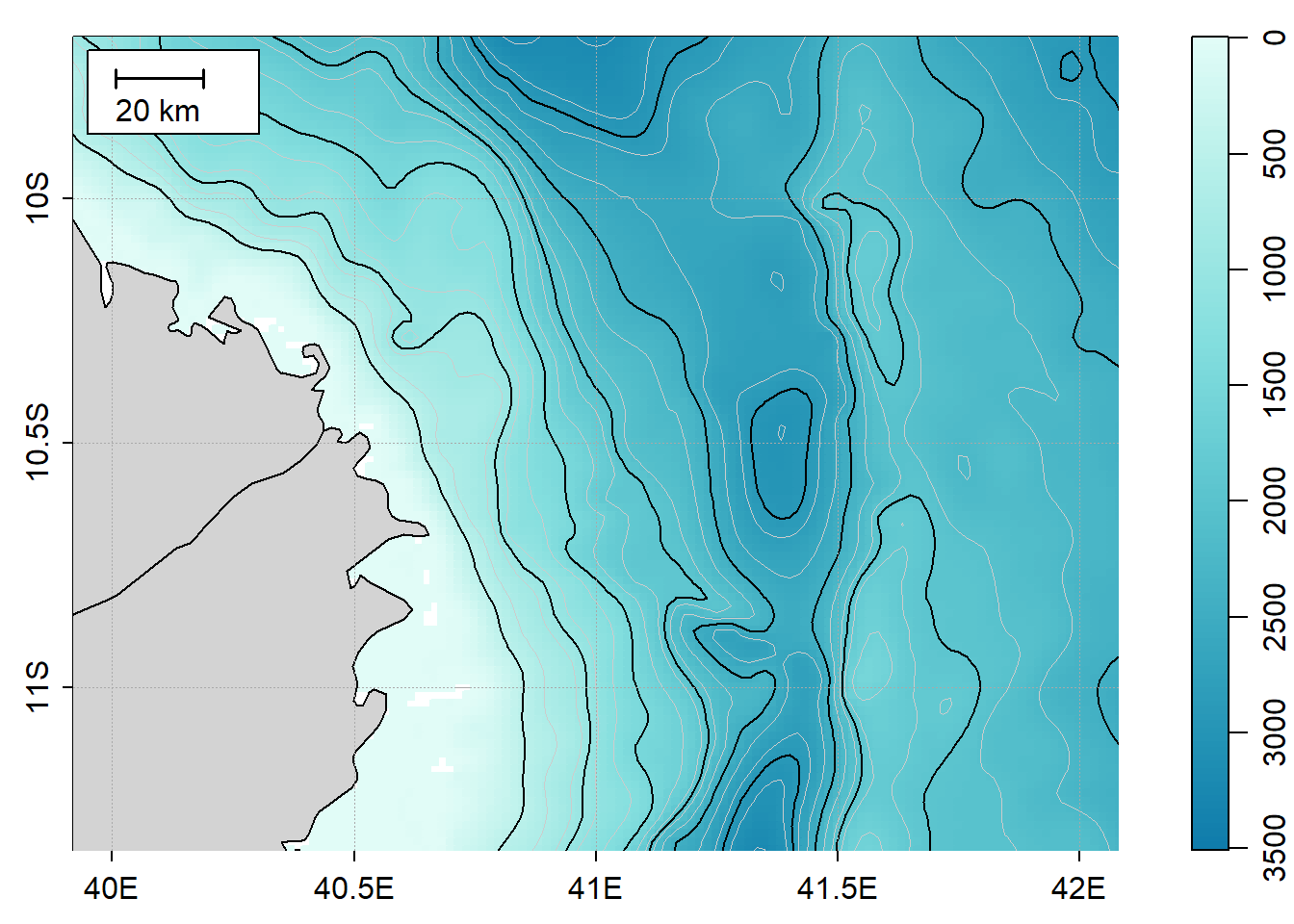
Figure 3: Bathymetry off Mtwara. the black line are contour at 500 m interval and the grey lines are contour at 200 m intervals
Reference
Kelley, Dan. 2015. Ocedata: Oceanographic Datasets for Oce. https://CRAN.R-project.org/package=ocedata.
Kelley, Dan, and Clark Richards. 2018. Oce: Analysis of Oceanographic Data. https://CRAN.R-project.org/package=oce.
R Core Team. 2018. R: A Language and Environment for Statistical Computing. Vienna, Austria: R Foundation for Statistical Computing. https://www.R-project.org/.