Isosurface of temperature, salinity, oxygen and fluorescence in Mafia Channel from CTD data

Iso surface

Often times we want to visualize the distribution of oceanographic variables across the space at specific depth. That kind of visualization refers to isosurface—layer(s) of constant values of another data variable, such as, constant depth. For this post highlights key steps to create isosurface from CTD profile data in Mafia channel. Because these channel is shallow with an average depth of 20 meters, we will calculate isosurface of f temperature, oxygen, fluorescene at the surface, 10 and 20 meters deep. Several packages are required to processes the CTD data and make isosurface. These packages include tidyverse for chaining the process and tidying of data (Wickham 2017); lubridate for manipulating date (Grolemund and Wickham 2011); oce for reading and processing CTD data (Kelley and Richards 2018) and sf for mapping (Pebesma 2018). The list of these packages are shown in the chunk below. Just load them using the require() function. You must have installed them in your machine before you load them.

require(tidyverse)
require(lubridate)
require(oce)
require(sf)

Location information

The CTD instrument used was not configured with a GPS. The latitude and longitude information at each cast was marked with a handheld GPS unit. These location information were downloaded with mapsource software and exported as comma separated file. The dataset was loaded into the workspace as shown in the chunk below.

station.tb = read_csv("./Wshark_raw data/cnv/stations.csv")

Then the path of the working directory in my local machine was defined. This is where the files for this post are stored.

mafia.files = dir("./Wshark_raw data/cnv/", pattern = ".cnv", full.names = TRUE)

The plotScan helped us identify the thresholds for cleaning the casts. This include removing all value in a profile measured above the sea surface pressure > 0, drop all values measured while the instrument was pulled out of the water and retain only the downcast records. Align the profile values to the standard depth of 0.25 meter interval. A for() loop was used to iterate and run through 40 CTD files. Each processed ctd profile was stored in the list file that was created before the looping. The chunk below show the code that processed the CTD data

mafia.ctd = list()

for (i in 1:length(mafia.files)){
  mafia.ctd[i] = read.ctd(mafia.files[i]) %>% 
    ctdTrim(method = "downcast") %>% 
    ctdDecimate(p = 0.25)%>%
    subset(pressure >= 0)
 
   mafia.ctd[[i]][["longitude"]] = station.tb$lon[i]
   mafia.ctd[[i]][["latitude"]] = station.tb$lat[i]
}

Three profiles were randomly selected and their temperature, and salinity profiles plotted against pressure as shown in figure 1. The chunk below show the code used to plot profiles in in figure 1.

par(mfrow = c(1,3))

for (k in c( 8,20,30)){

plot(mafia.ctd[[k]], which = 1)
plotInset(xleft =  min(mafia.ctd[[k]][["salinity"]], na.rm = TRUE),
          ybottom =  max(mafia.ctd[[k]][["pressure"]]), 
          xright =  max(mafia.ctd[[k]][["salinity"]], na.rm = TRUE), 
          ytop = max(mafia.ctd[[k]][["pressure"]])/2, 
          expr = plot(mafia.ctd[[k]], 
                      which = "map", 
                      coastline = "coastlineWorldFine",
                      span=50, 
                      mar=NULL, cex.axis=3/4))

}

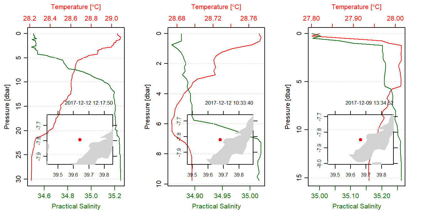
Figure 1: Profiles of selected CTD cast. An inset map show the location of the cast in the Mafia channel

make a data frame from CTD list

The mafia.ctd is the list file with 40 CTD cast. We need to convert the profile value of each cast to data frame and then combine them to form a large data frame with all the cast embeded. That is tedious to do it manually. However, we can tell R to do it for us using a for() loop function. The chunk below highlight the iterated code for the process

ctd.tb = list()

for (j in 1:length(mafia.ctd)){
  
ctd.tb[[j]] = mafia.ctd[[j]]@data %>% 
  as.tibble() %>% 
  mutate(lon = mafia.ctd[[j]]@metadata$longitude,
         lat = mafia.ctd[[j]]@metadata$latitude,
         scientists = mafia.ctd[[j]]@metadata$scientist,
         time = station.tb$Date[j] %>% dmy(),
         profile = j, 
         scientists = "Patroba Matiku, Baraka Kuguru & Masumbuko Semba") %>%
  select(time, lon,lat, scientists, profile, pressure, depth, 
         temperature, salinity, conductivity, oxygen, fluorescence)

}

ctd.df = ctd.tb %>% bind_rows()

Figure 2 is a map of Mafia channel showing the location where profiles of temperature, salinity, oxygen, and fluorescene were measured against the water column (depth).

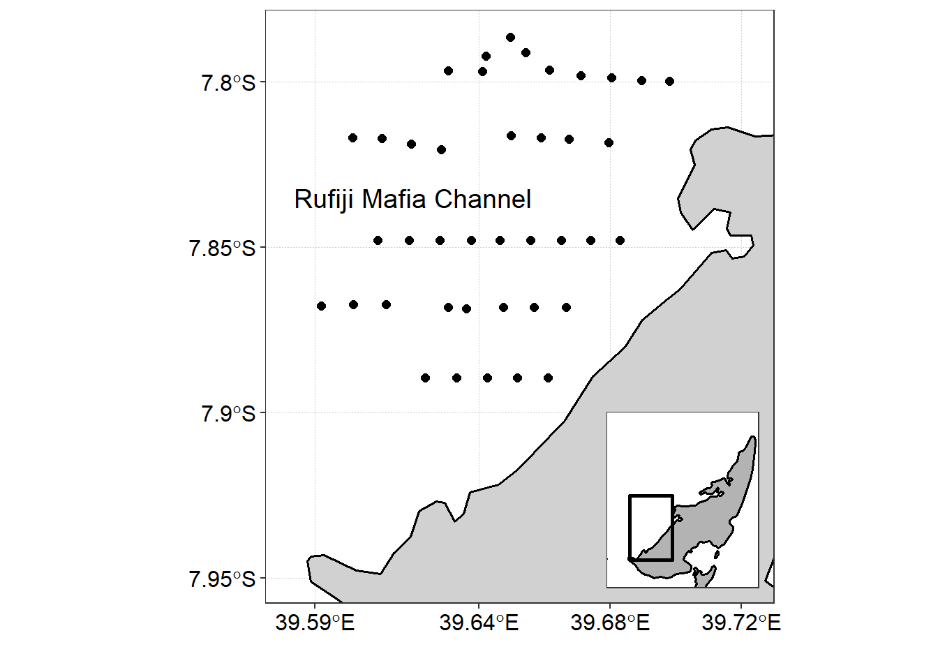
Figure 2: CTD cast in the Mafia Channel

Isosurface in Mafia Channel

Once we have the data frame of each ctd cast, we can make isosurface at three different depth—surface, 10 and 20 meter. Because the profiles were measured at randomly locations, we need to grid them and make the distribution evenly. The interpBarnes() function from oce package was used for gridding the unevenly distributed ctd points. We looped the procedure with for() function. The loop does three main things— select the depth; extract the x = longitude,y = latitude ,z = variable from the filtered depth—surface; 10 or 20; and interpolate the variables to the specific longitude and latitude. The chunk below highlights the codes used to create an isosurface of temperature shown in figure 3. Similar technique was used to make isosurface of oxygen (Figure 4); salinity (Figure 5) and fluorescence (Figure 6).

depth = c(0.25,10,20)

par(mfrow = c(1,3))

for (m in depth){
  
surface = ctd.df %>% filter(pressure == m)
x = surface$lon
y = surface$lat
z = surface$temperature

interp.temp = interpBarnes(x = x, 
                           y = y, 
                           z = z, 
                           xg = pretty(x, n = 50) , 
                           yg = pretty(y, n = 50))

imagep(interp.temp$xg, interp.temp$yg, interp.temp$zg, filledContour = TRUE, 
       col = oce.colors9A(120), main = paste("Depth = ", m, "meters"), zlim = c(27.8,29))
contour(interp.temp$xg, interp.temp$yg, interp.temp$zg, col = "black", add = TRUE)

}

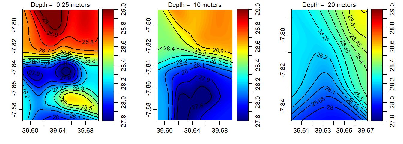
Figure 3: The spatial distribution of temperature in the Mafia channel at the surface (left panel); 10 m deep (middle panel) and 20 m deep (right panel

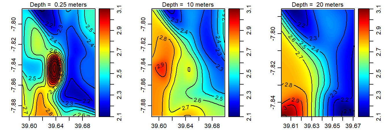
Figure 4: The spatial distribution of oxygen in the Mafia channel at the surface (left panel); 10 m deep (middle panel) and 20 m deep (right panel

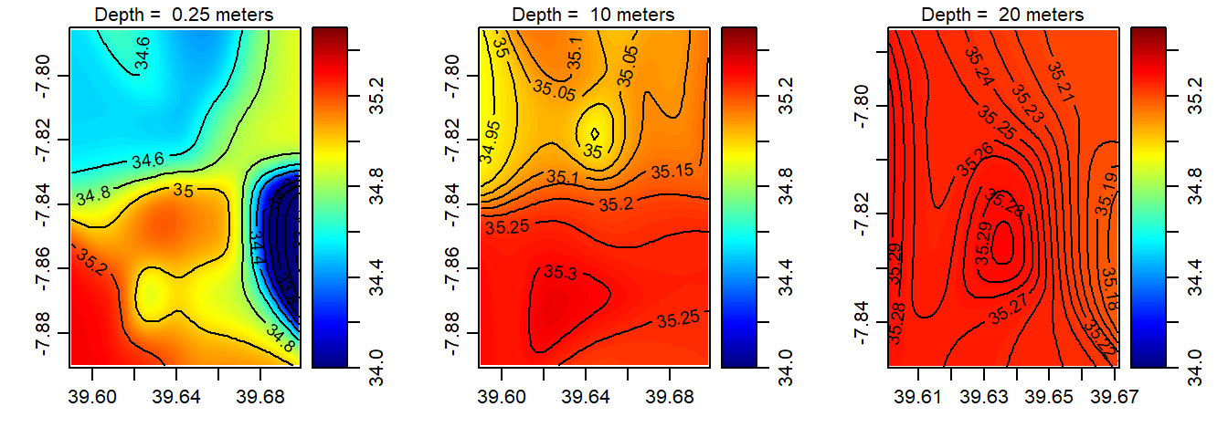
Figure 5: The spatial distribution of salinity in the Mafia channel at the surface (left panel); 10 m deep (middle panel) and 20 m deep (right panel

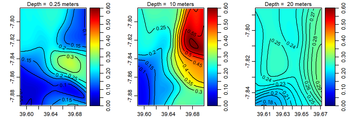
Figure 6: The spatial distribution of fluorescence in the Mafia channel at the surface (left panel); 10 m deep (middle panel) and 20 m deep (right panel

References

Grolemund, Garrett, and Hadley Wickham. 2011. “Dates and Times Made Easy with lubridate.” Journal of Statistical Software 40 (3): 1–25. http://www.jstatsoft.org/v40/i03/.
Kelley, Dan, and Clark Richards. 2018. Oce: Analysis of Oceanographic Data. https://CRAN.R-project.org/package=oce.
Pebesma, Edzer. 2018. Sf: Simple Features for R. https://CRAN.R-project.org/package=sf.
Wickham, Hadley. 2017. Tidyverse: Easily Install and Load the ’Tidyverse’. https://CRAN.R-project.org/package=tidyverse.