Comparing classical methods for estimating the mixed layer depth along the transect off Kimbiji, Tanzania

Introduction

Upper Ocean is characterized for a quasi-homogeneous layer where temperature, salinity and density almost constant with increasing depth (Costoya et al. 2014). This homogeneity layer is caused by turbulent vertical mixing that is driven by heat loss from the ocean to the atmosphere, as well as by wind stress (Stranne et al. 2018). The deepest layer affected by this turbulent mixing is called mixed layer depth (MLD), which marks the width of the upper ocean that interacts with the atmosphere (Kelley 2018).

The depth of the mixed layer (MLD) influences the exchange of heat and gases between the atmosphere and the ocean and constitutes one of the major factors controlling ocean primary production as it affects the vertical distribution of biological and chemical components in near-surface waters. Estimation of the MLD are often made by means of conductivity, temperature and depth (CTD) casts (Stranne et al. 2018). However, there different techniques are used and there is little agreement on which technique is the best for estimating MLD (Kelley 2018). In this post I illustrate the classical three approaches that are widely used to estimate the MLD.

A first group of the methods involves estimating the thickness of a near-surface region within which water properties are nearly constant. I dub this approach as criterion because it base on the criteria to estimate the MLD. For example, the MLD may be defined as the shallowest depth at which density or temperature differs from the surface value by a fixed amount \(\Delta \rho\) or \(\Delta \Theta\). Costoya et al. (2014) reported a temperature ranged 0.1–1.0^oC and density of 0.125 kgm^-3 are commonly thresholds used in this approach. A second group of methods involves derivatives of water properties, based on, e.g., \(\delta \Theta\)/\(\delta z\). For example, the thermocline could be inferred as the spot where |\(\delta \Theta\)/\(\delta z\)| is largest, with the region above being interpreted as a mixed layer (Kelley 2018). The third method use optimal fitting to estimate the MLD.

If you find yourself left out in this post, I have described these method in the previous post. For detail of the criterion, check this post. For a length procedure of the derivatives method, check on this post and the optimal technique is discussed in this post. I only need to load the oce package developed by Kelley and Richards (2018) and tidyverse package developed by Wickham (2017) for this post. If you have not installed these packages in your machine, stop here and install them first. You may also load the ocedata package (Kelley 2015). But you can finish this task without it.

require(oce)
require(ocedata)
require(tidyverse)

Dataset

To illustrate the concept of estimating the Mixed Layer Depth (MLD) of the upper ocean off coastal of Kimbiji, Tanzania, I used the ctd data collected in August 2004 with Algoa. To make easy to process the dataset, we first use the function dir() to read names of downcast files from the local directory . We limit file names by parsing the pattern argument in the function. Because the local directory is not in the working directory, we also parse the full.names() function as the argument that will give the full path of the files.

Because there are several ctd cast, the for() function was used to iterate the process of reading the ctd files. Before looping, an empty list files was created to store profile data of each ctd cast. Note that the process is pipped with the pipe operator (%>%). Pipping is important because it reduce the processing time and also avoid creation of intermediate files during the process. It also make writing and reading code easier than the traditional syntax.

algoa.list = list()

for (i in 1:length(algoa)){
  
  algoa.list[[i]] = algoa[i] %>% read.ctd()
}

Then the hydrographic section was created with as.section() fuction. This function requires the ctd cast are in list format—which was done in the above section. Once the section was created, the ctd profiles outside the selected transect covering the Kimbiji water were dropped using the subset() function. Figure 1 present the transect with the temperature, oxygen and fluorescence section off the Kimbiji.

## Make a section of all ctd casts
algoa.section = algoa.list %>% as.section()

## subset the section for ctd along the Kimbiji only
kimbiji.section = algoa.section %>% subset(latitude > -7.2 & latitude < -7)

## plot cross section with a map along the transect of Kimbiji
kimbiji.section %>%
  sectionGrid(p = seq(0,300,5)) %>%
  sectionSmooth() %>%
  plot(xtype = "longitude", which = c("map", "temperature", "oxygen", "fluorescence"), ylim = c(200,5), ztype = "image")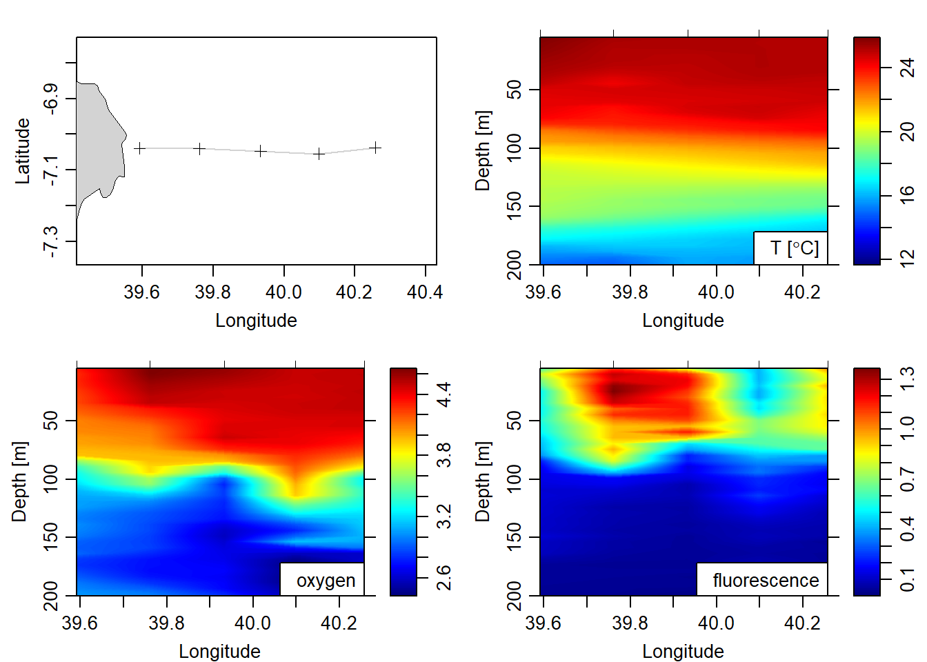

Figure 1: Cross section of the transect off Kimbiji

Estimating Mixed Layer Depth

The method for estimating the Mixed Layer depth use individual profile of the ctd cast, therefore, the section of Kimbiji was converted to a list file. The chunk below show one line that accomplish conversion of section to list with just a double curl brackets.

# make a list file of the section from Kimbiji
kimbiji.ctd.list = kimbiji.section[["station"]]

The criterion method

The criterion method codes are presented in the chunk below. In a nutshell, the procedure process the mld for each cast, store them in the list file, plot the temperature profile and insert its corresponding MLD. All these steps are done within a loop for the five cast along this transect. Once the loop is terminated, in the same chunk the list file that contain MLD is converted to a data frame. Figure 2 presents the estimated MLD for each CTD cast off-Kimbiji transect.

## criterion
mld.criterion = list()

par(mfrow = c(2,3))

for (i in 1:length(kimbiji.ctd.list)){
  # readline(prompt = "ENTER")
  ctd = kimbiji.ctd.list[[i]]
  ctd = ctd %>% subset(pressure > 10)
 

      temperature = ctd[["temperature"]]
      pressure = ctd[["pressure"]]
  
    for (criterion in 0.5){
      inMLD =  abs(temperature[1] - temperature) < criterion
      MLDindex = which.min(inMLD)
      MLDpressure = pressure[MLDindex]
      
        ctd %>% plotProfile(xtype = "temperature", ylim = c(150,20))
        abline(h = pressure[MLDindex], lwd = 2, lty = "dashed")
        
       
        mld.criterion[i] = MLDpressure

    }
}

mld.criterion = mld.criterion %>% 
  as.data.frame() %>% t() %>% 
  as.tibble()%>%  
  rename(criterion = V1)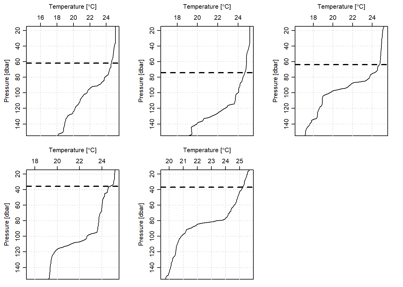 

Figure 2: Mixed Layer Depth estimated from criterion method for five CTD casts off-Kimbiji transect

The derivative method

The chunk below highlight how to estimate the MLD with the derivative method. Each cast MLD is stored in the list file and then converted into data frame. Figure 3 presents the estimated MLD for each CTD cast off-Kimbiji transect.

## derivative

pstar.mld = list()

par(mfrow = c(2,3))

for (j in 1:length(kimbiji.ctd.list)){
  
  # readline(prompt = "ENTER")
  
  ctd = kimbiji.ctd.list[[j]]
  ctd = ctd %>% subset(pressure > 10)
  temperature = ctd[["temperature"]]
  pressure = ctd[["pressure"]]
  mid = which.max(swN2(ctd))
  pstar = pressure[mid]
  pstar.mld[j] = pstar
  
    # plotProfile(ctd, xtype = "N2", ylim = c(150,20))
    # abline(h = pstar, lwd = 1, lty = 2)
    
    plotProfile(ctd, xtype = "temperature", ylim = c(150,20))
    abline(h = pstar, lwd = 2, lty = 2)
    
    # plotProfile(ctd, xtype = "salinity", ylim = c(150,20))
    # abline(h = pstar, lwd = 1, lty = 2)
}

## Convert the list file into data frame
mld.derivative = pstar.mld %>%
  as.data.frame() %>%
  t() %>%
  as.tibble() %>%
  rename(derivative = V1)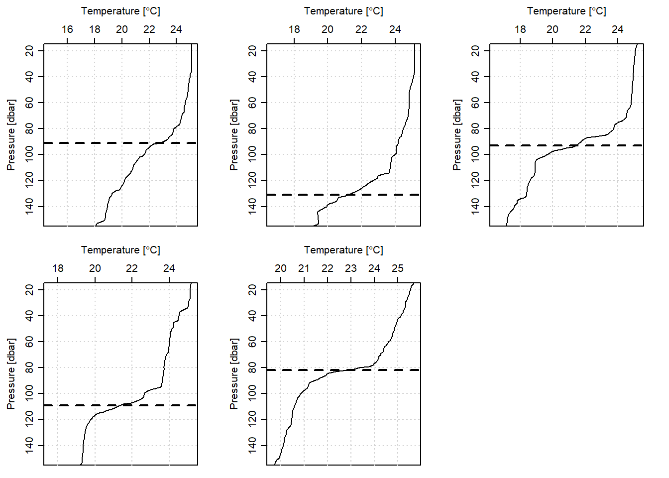

Figure 3: Mixed Layer Depth estimated from derivative method for five CTD casts off-Kimbiji transect

The Optimal Linear fitting Method

The optimal method was first developed by Chu and Fan (2010). The chunk below highlights the codes for a function developed in R programming languages for estimating the MLD from CTD profiles.

MLDchu = function(ctd, n = 5, variable = "temperature")
{
  pressure = ctd[["pressure"]]
  x = ctd[[variable]]
  ndata = length(pressure)
  E1 = rep(NA, ndata)
  E2 = E1
  E2overE1 = E2
  kstart = min(n,3)
  for (k in seq(kstart, ndata-n,1)){
    above = seq.int(1,k)
    below = seq.int(k+1, k+n)
    fit = lm(x~pressure, subset = above)
    E1[k] = sd(predict(fit) - x[above])
    pBelow = data.frame(pressure = pressure[below])
    E2[k] = abs(mean(predict(fit, newdata = pBelow) -x[below]))
    E2overE1[k] = E2[k] / E1[k]
    
  }
  
  MLDindex = which.max(E2overE1)
  return(list(MLD = pressure[MLDindex], MLDindex = MLDindex, E1 = E1, E2 = E2))
  
}

Once we have written the MLDchu() function, then estimating the MLD for each cast is done with the code in the chunk below. Figure 4 presents the estimated MLD for each CTD cast off-Kimbiji transect.

lon = kimbiji.section[["longitude"]] %>% unique()
lat = kimbiji.section[["latitude"]] %>% unique()

## preallocate the list file that will store mld value
mld.optimal = list()

## make subplots 
par(mfrow = c(2,3))
## loop the process
for (j in 1:length(kimbiji.ctd.list)){
  ## get the ctd value of the station
ctd = kimbiji.ctd.list[[j]] %>% ctdDecimate(p = seq(8,150,10))

## compute the mld of each station
mld = MLDchu(ctd)
mld.optimal[j] = mld$MLD

## draw a profile of the ctd cast
plotProfile(ctd, xtype = "temperature")
## add a line showing the mld
abline(h = mld$MLD, lwd = 2, lty = "dashed")

}

## convert the mld list into tibble
mld.optimal = mld.optimal%>% as.data.frame() %>% t() %>% as.tibble() %>% rename(optimal = 1)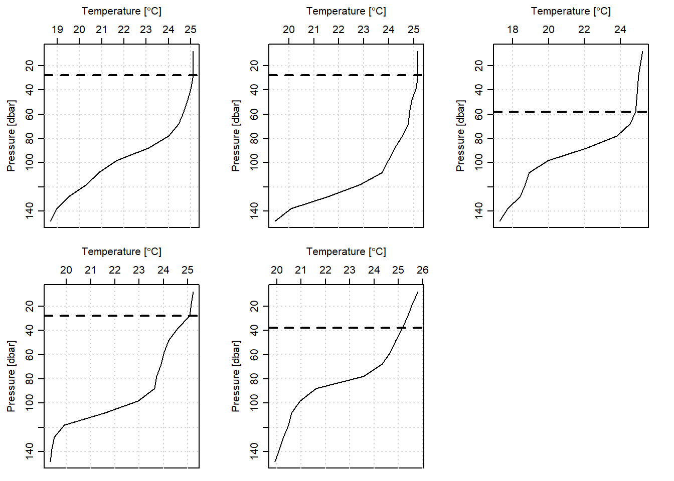

Figure 4: Mixed Layer Depth estimated from optimal method for five CTD casts off-Kimbiji transect

Lastly, the mld values from optimal, criterion and derivatives method were stitched together with longitude and latitude, which help us to compare the value of the MLD (Table ??).

mld.all = data.frame(lon,lat, mld.criterion, mld.derivative, mld.optimal)

mld.all  %>% 
  kableExtra::kable(format = "html", digits = 2,col.names = c("Longitude", "Latitude", "Criterion", "Derivative", "Optimal"), caption = "Mixed Layer Depth estimated from different methods", align = "c") %>%
  kableExtra::column_spec(column = 1:5, width = "3cm", color = "black") %>%
  kableExtra::add_header_above(c("Cast Location" = 2, "MLD Methods" = 3))

Table 1: Mixed Layer Depth estimated from different methods

Cast Location		MLD Methods
Longitude	Latitude	Criterion	Derivative	Optimal
40.26	-7.04	62	91	28
40.10	-7.05	74	131	28
39.93	-7.05	64	93	58
39.76	-7.04	36	109	28
39.59	-7.04	37	82	38

Figure 5 is the cross section of temperature superimposed with the lines plots for the three classical methods for estimating the MLD. This figures clearly indicate the deep MLD is from the derivative method followed by the criterion and the optimal method has the shallower MLD. The other clear observation is that the optimal MLD vary toward offshore (Figure 5). In contrast, the derivative and criterion method, though have different values at each cast, they both show the MLD is getting deeper toward offshore (Figure 5)

par(mfrow = c(1,3))

## temperature section
kimbiji.section %>%
  sectionGrid(p = seq(0,300,2)) %>%
  # sectionSmooth() %>%
  plot(xtype = "longitude", which = "temperature", ylim = c(200,4), ztype = "image", zlim = c(20,26), zclip = TRUE)

lines(x = mld.all$lon , y = mld.all$criterion, lwd =2, lty = 2)
lines(x = mld.all$lon , y = mld.all$derivative, lwd =2, lty = 3)
lines(x = mld.all$lon , y = mld.all$optimal, lwd =2, lty = 1)

## density section
kimbiji.section %>%
  sectionGrid(p = seq(0,300,2)) %>%
  # sectionSmooth() %>%
  plot(xtype = "longitude", which = "density", ylim = c(200,4), ztype = "image")

lines(x = mld.all$lon , y = mld.all$criterion, lwd =2, lty = 2)
lines(x = mld.all$lon , y = mld.all$derivative, lwd =2, lty = 3)
lines(x = mld.all$lon , y = mld.all$optimal, lwd =2, lty = 1)


## fluorescence section
kimbiji.section %>%
  sectionGrid(p = seq(0,300,2)) %>%
  # sectionSmooth() %>%
  plot(xtype = "longitude", which = "fluorescence", ylim = c(200,4), ztype = "image")

lines(x = mld.all$lon , y = mld.all$criterion, lwd =2, lty = 2)
lines(x = mld.all$lon , y = mld.all$derivative, lwd =2, lty = 3)
lines(x = mld.all$lon , y = mld.all$optimal, lwd =2, lty = 1)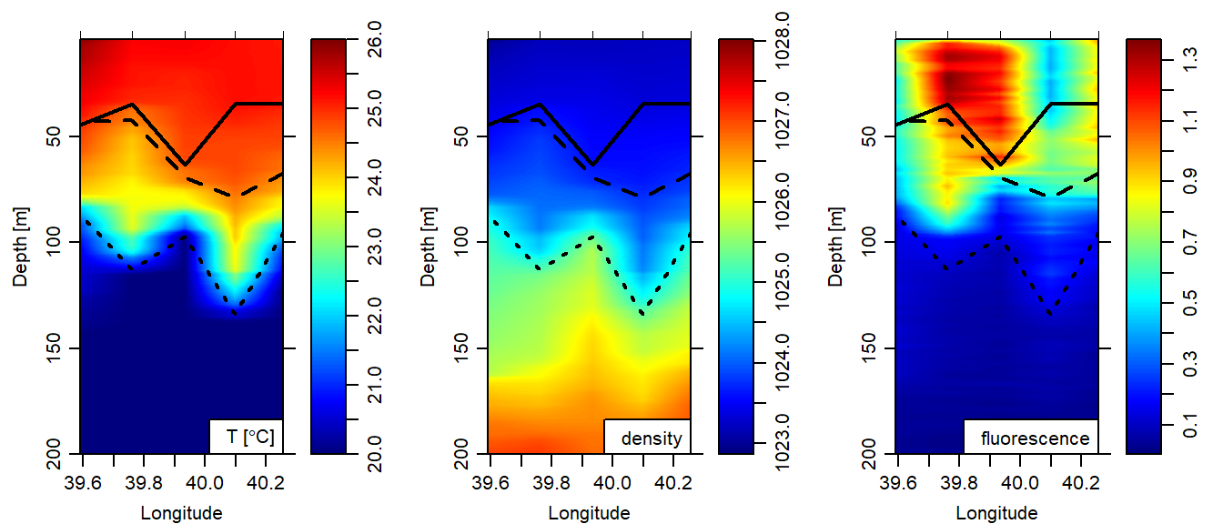

Figure 5: Method for detecting the Mixed Layer Depth overlaid on cross section of temperature (left panel), density (middle panel) and fluorescence (right panel). The bold black line is the optimal, the dashed line is the criterion and and the dotted line represent the derivative method