Detecting Mixed Layer Depth with Optimal Linear fitting method.

Introduction

The mixed layer is a thin layer with constant temperature and salinity from the surface down to a depth where the values differ from those at the surface (Boyer Montégut et al. 2004). Wind blowing on the ocean stirs the upper layers leading to a thin mixed layer (Stewart 2008). The resulting surface mixed layer is important for local primary production, climate and ocean circulation (Kelley 2018). Although the mixed layer is an important oceanographic parameter, there different approaches that are used and each method depends on the scientific application.

The two classic methods are criterion and derivative explained in tha last two post in this blog. In this post I explain the third method developed by Chu and Fan (2010). This method use an optimal linear fitting to determine the mixed layer depth. Using similar approach, Kelley (2018) wrote a function in R programming language that returns the mixed layer depth and other interesting elements of the calculations. The chunk below highlight the key steps of the function. The argument n determines the number of data levels to examine below the focus depth and the variable argument determine the hydrographic variable that will be used for estimation, the default is temperature.

MLDchu = function(ctd, n = 5, variable = "temperature")
{
  pressure = ctd[["pressure"]]
  x = ctd[[variable]]
  ndata = length(pressure)
  E1 = rep(NA, ndata)
  E2 = E1
  E2overE1 = E2
  kstart = min(n,3)
  for (k in seq(kstart, ndata-n,1)){
    above = seq.int(1,k)
    below = seq.int(k+1, k+n)
    fit = lm(x~pressure, subset = above)
    E1[k] = sd(predict(fit) - x[above])
    pBelow = data.frame(pressure = pressure[below])
    E2[k] = abs(mean(predict(fit, newdata = pBelow) -x[below]))
    E2overE1[k] = E2[k] / E1[k]
    
  }
  
  MLDindex = which.max(E2overE1)
  return(list(MLD = pressure[MLDindex], MLDindex = MLDindex, E1 = E1, E2 = E2))
  
}

Packages

Once we have the function, we can process the ctd data and estimate the MLD for each profile. We rely on oce (Kelley and Richards 2018) and tidyverse (Wickham 2017) packages for this routine. We load these packages into the workspace using the require(). If you have not installed these packages in your machine, please go ahead and install them from the CRAN.

require(oce)
require(ocedata)
require(tidyverse)

Dataset

We use the ctd data collected in August 2004 with Algoa to demonstrate the process. The dataset cover the four transects along the coastal water of Tanzania (Figure 1). To make easy to process the dataset, we first use the function dir() to read names of downcast files from the local directory . We limit file names by parsing the pattern argument in the function. Because the local directory is not in the working directory, we also parse the full.names() function as the argument that will give the full path of the files.

## similar to the chunk above, but this will act as front end, not process anything
algoa = dir(path = "./ctd_algoa/", pattern = "dstn", full.names = TRUE)

Processing the CTD dataset

Using the for() function to iterate the process of reading the ctd files. Before we loop, an empty list files was created that will store profile data for each ctd cast. Note that the process is chained with the pipe operator (%>%)—pipping. Pipping is important because it reduce the processing time and also avoid creation of intermediate files during the process. It also make writing and reading code easier than the traditional syntax.

algoa.list = list()

for (i in 1:length(algoa)){
  
  algoa.list[[i]] = algoa[i] %>% read.ctd()
}

## Make a section and plot a map that show the location of each profile

algoa.section = algoa.list %>% as.section()

algoa.section %>% plot(which = "map")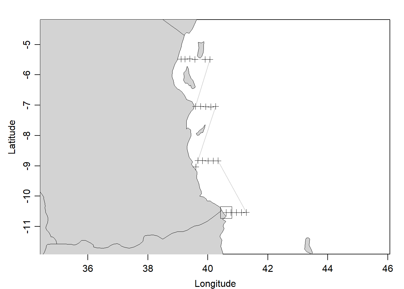

Figure 1: a sketch map showing the CTD cast along the sections

Estimate the MLD of Pemba transect

For illustration, we picked only CTD profiles measured along the transect located between the Unguja and Pemba Island shown in. You can easily notice from figure 1 that the transect contain profiles recorded above latitude 06^oS. Because we had already created a MLDchu() function, we use it to determine the MLD of each profile (Figure 2). The chunk below highlight the steps of estimating the MLD

## pick profile for pemba transect only, which are above latitude 
pemba.section = algoa.section %>% subset(latitude >-6) 

## convert the section into the list
pemba.list = pemba.section[["station"]]

lon = pemba.section[["longitude"]] %>% unique()
lat = pemba.section[["latitude"]] %>% unique()

## preallocate the list file that will store mld value
mld.pemba = list()

## make subplots 
par(mfrow = c(2,3))
## loop the process
for (j in 1:length(pemba.list)){
  ## get the ctd value of the station
ctd = pemba.list[[j]] %>% ctdDecimate(p = seq(8,150,10))

## compute the mld of each station
mld = MLDchu(ctd)
mld.pemba[j] = mld$MLD

## draw a profile of the ctd cast
plotProfile(ctd, xtype = "temperature", main = j)
## add a line showing the mld
abline(h = mld$MLD, lwd = 2, lty = "dashed")

}

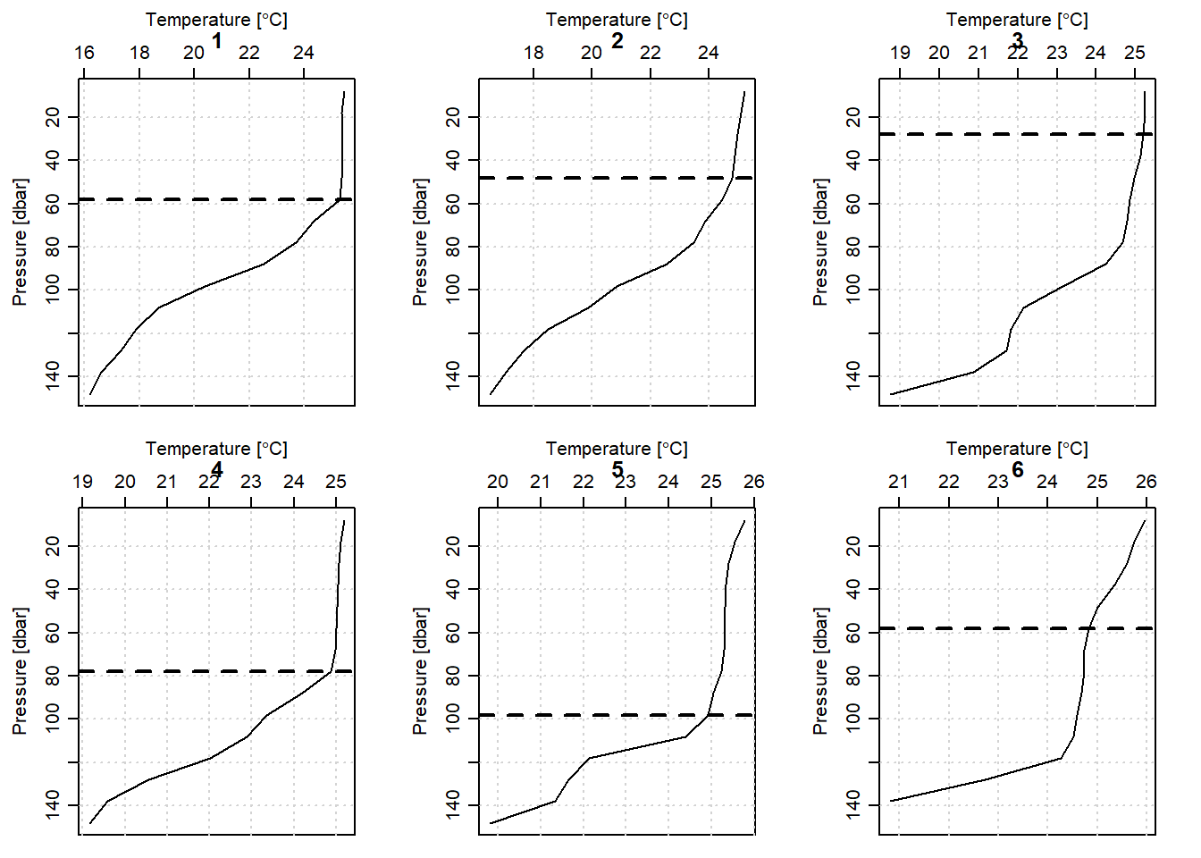
Figure 2: Mixed layer depth of the six profile along the transect within Unguja and Pemba Islands

Make data frame of the MLD

To overlay the MLD over the hydrographic section, the list containing the mld was transformed into individual vector and combined with longitude and latitude information. This process create a data frame that show both the location and the mld at each cast. The chunk below highlight the steps involved to make this data frame. Figure 3 show the cross of temperature along the pemba transect. The white dotted line indicate the mixed layer depth along the transect.

## convert the mld list into tibble
mld.pemba.tb = mld.pemba%>% as.data.frame() %>% t() %>% as.tibble() %>% rename(mld = 1)

## bind the mld with longitude and latitude information
mld.pemba.df = data.frame(lon,lat, mld.pemba.tb )

par(mfrow = c(1,2))
## draw a section of the pemba
pemba.section %>% plot(which = "temperature", ztype = "image", ylim = c(200,0), 
                       xtype = "longitude", zcol = oceColors9A(120))
## add the mld into the section
lines(x = mld.pemba.df$lon, y = mld.pemba.df$mld, col = "white", lwd = 2, lty = "dashed")

## draw a contour section of the pemba
pemba.section %>% plot(which = "temperature", ztype = "contour", ylim = c(200,0), 
                       xtype = "longitude")
## add the mld into the section
lines(x = mld.pemba.df$lon, y = mld.pemba.df$mld, col = "black", lwd = 2, lty = "dashed")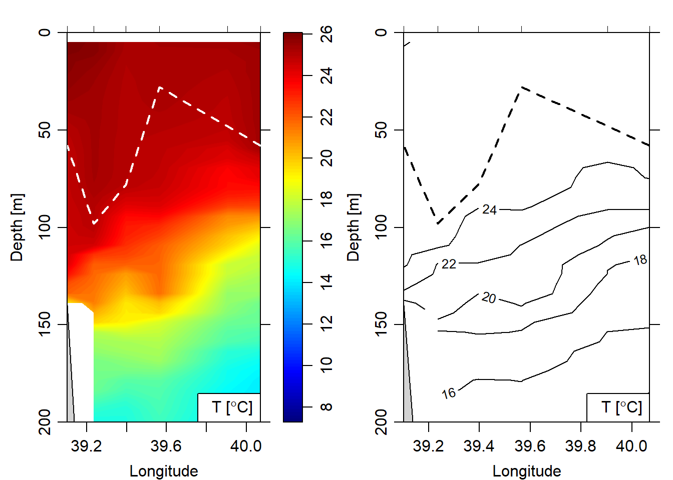

Figure 3: Mixed layer depth (white color) overlaid on the temperature cross section image (left panel) and contour (right panel)

Conclusion

We have seen the criterion and derivative approaches in the previous post. This post mark the third method—optimal linear fitting.Unlike the other two methods, this technique returns not just the mixed layer depth, but also some other interesting elements of the calculation.

References

Boyer Montégut, Clément de, Gurvan Madec, Albert S Fischer, Alban Lazar, and Daniele Iudicone. 2004. “Mixed Layer Depth over the Global Ocean: An Examination of Profile Data and a Profile-Based Climatology.” Journal of Geophysical Research: Oceans 109 (C12). Wiley Online Library.
Chu, P, and C. Fan. 2010. “Optimal Linear Fitting for Objective Determination of Ocean Mixed Layer Depth from Glider Profiles.” Journal of Atmospheric and Oceanic Technology 27 (11): 1893–8.
Kelley, Dan. 2018. “R Tutorial for Oceanographers.” In Oceanographic Analysis with R, 5–90. Springer.
Kelley, Dan, and Clark Richards. 2018. Oce: Analysis of Oceanographic Data. https://CRAN.R-project.org/package=oce.
Stewart, Robert H. 2008. Introduction to Physical Oceanography. Book. Robert H. Stewart.
Wickham, Hadley. 2017. Tidyverse: Easily Install and Load the ’Tidyverse’. https://CRAN.R-project.org/package=tidyverse.