Introduction

In the previous post, I illustrate how to detect the mixed layer depth (MLD) with the change in temperature criterion approach (\(\Delta T\)). In this post I explain how to detect the MLD using derivatives of water properties based \(\delta T/ \delta z\). With this approach, the thermocline can be detected at a depth where \(\delta T/ \delta z\) is larges, with the region above considered as the mixed layer depth. Despite its simplest in detecting the MLD, this approach has its disadvantage that the profile data has to be smoothed, which can lead to over or under–estimate the MLD. D. Kelley and Richards (2018) developed a swN2() function that handle the smoothing shown in equation (1)

\[ \begin{equation} N^2 = - \frac{g \delta \rho}{\rho \delta z} \tag{1} \end{equation} \]

As before, we need to load the necessary packages into the workspace required for importing, processing argo dataset, and displaying results.

require(tidyverse)
require(oce)
require(ocedata)
require(sf)
require(lubridate)

argo.float = argo[39]%>% 
  read.argo()%>% 
  handleFlags() %>% 
  argoGrid(p = seq(5,400,5))

time = argo.float[["time"]]
lon = argo.float[["longitude"]]
lat = argo.float[["latitude"]]

argo.section = argo.float%>%  
  as.section()

subset the EACC from the dataset

The section provide a nifty way to subset only the profile we are interested. I did a simple exploration and found that the profile number 206 to 212 cover well the EACC. Therefore, we only pick these profile and drop the rest from the dataset. Because I also need to know the time of each profile, I selected the time and location information using the index method and make a data frame of these information. Figure ?? show the location of the profile and the time in which the measurement were done and figure 2 hydrographic section of these station to 200 meter deep

## make a section from list of argo profile
eacc.section = argo.section %>% subset(stationId  >= 206 & stationId <= 212)

## obtain the time and spatial information corresponding to each profile
time.eacc = time[206:212] %>% as.Date()
lon.eacc = lon[206:212]
lat.eacc = lat[206:212]

## create a table from the time, lon and lat variable extracted above
eacc.extract.tb = data.frame(time.eacc, lon.eacc, lat.eacc) %>% 
  rename(time = 1, lon = 2, lat = 3)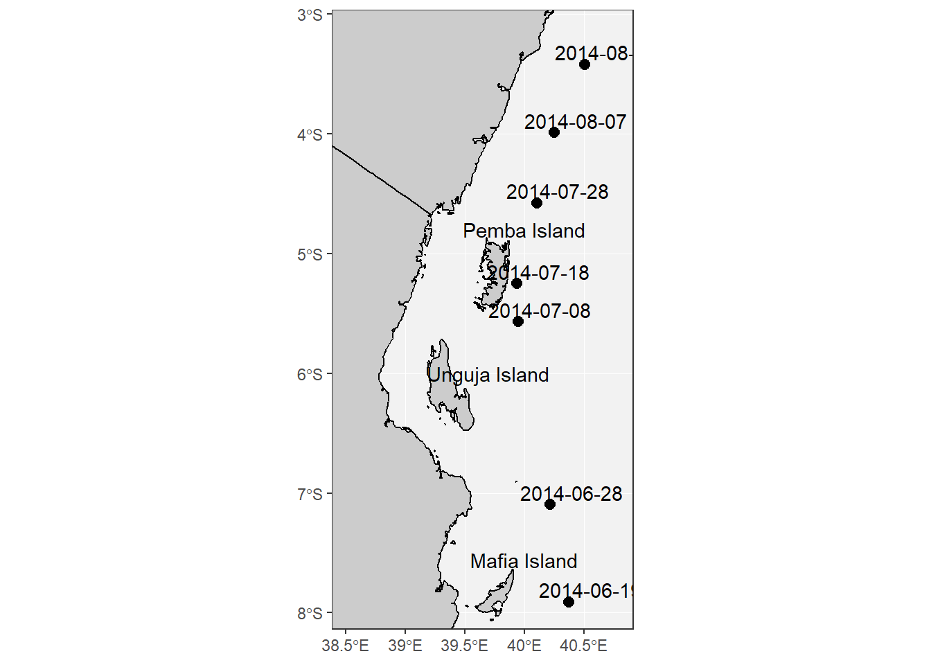

Figure 1: Map of the East African Coast showing the location of the Argo float profiles and the date the records were measured

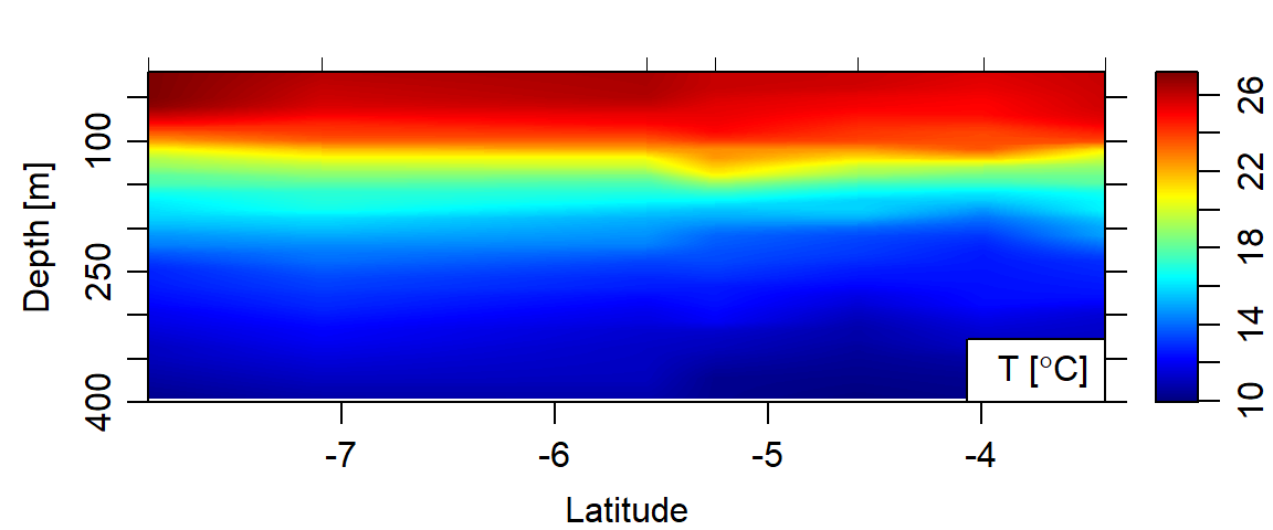
Figure 2: Hydrographic section of temperature

The code for derivative determination of MLD

The mathematical procedure used to detect MLD with the derivative detection show in in figure 3 is created with code in the chunk below.

stations = eacc.section[["station"]]

pstar.mld = list()

par(mfrow = c(2,4))

for (j in 1:length(stations)){
  
  # readline(prompt = "ENTER")
  
  ctd = stations[[j]]
  ctd = ctd %>% subset(pressure > 10)
  temperature = ctd[["temperature"]]
  pressure = ctd[["pressure"]]
  mid = which.max(swN2(ctd))
  pstar = pressure[mid]
  pstar.mld[j] = pstar
  
    # plotProfile(ctd, xtype = "N2", ylim = c(150,20))
    # abline(h = pstar, lwd = 1, lty = 2)
    
    plotProfile(ctd, xtype = "temperature", ylim = c(150,20))
    abline(h = pstar, lwd = 1, lty = 2)
    
    # plotProfile(ctd, xtype = "salinity", ylim = c(150,20))
    # abline(h = pstar, lwd = 1, lty = 2)
}

pstar.mld = pstar.mld %>%
  as.data.frame() %>%
  t() %>%
  as.tibble() %>%
  rename(mld = V1)

pstar.mld = eacc.extract.tb %>% bind_cols(pstar.mld)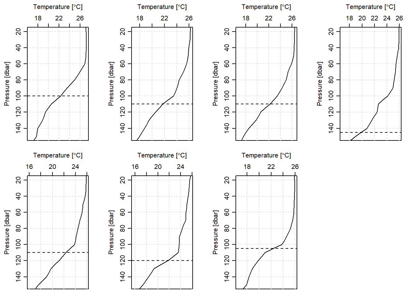

Figure 3: Mixed Layer Depth (MLD) for the seven profiles along the East African Coastal Current

Conclusion

D. E. Kelley (2018) explained that although the mixed-layer depth (MLD) is a parameter of great interest, there is little agreement on how it should be defined. This is partly because the most appropriate definition can depend on the scientific application. This is clearly illustrated in figure 4 that shows the discrepancy of the two approaches, with the derivative method giving a deeper MLD compared to the criterion method.

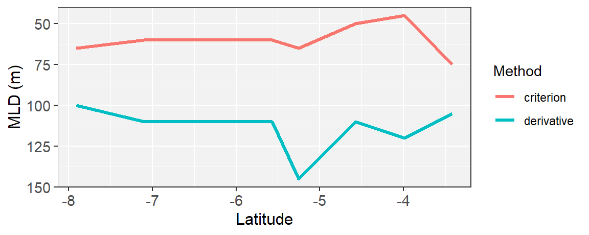
Figure 4: Comparison of two methods for inferring mixed-layer depth. Red line: based on Conservative Temperature, with mixed-layer depths inferred using temperature criterion of 0.1 0.5 C Pale green.: based on the peak of N2 derivative.