Introduction
The ocean mixed layer is narrow band of the suface water that is homogenous—where temperature, salinity and density scarcely vary with increasing depth (Costoya et al. 2014). This homogeneity layer is caused by turbulent vertical mixing that is driven by heat loss from the ocean to the atmosphere and wind stress. The deepest layer affected by this turbulent mixing is called mixed layer depth (MLD), which marks the width of the upper ocean that interacts with the atmosphere. The aim of this post is determine the MLD along the path of the East African Coastal Current. We use the Argo float dataset that contain the profile of temperature and salinity from the surface down to two kilometer deep.
I use R programming language as an environment for the required routine to calculate the MLD (R Core Team 2018). To accomplish this process I need several packages. You can achieve the process just by relying on the base R. but, Kelley and Richards (2018) developed oce package that makes R programming languages (R Core Team 2018) capable of handling and analysing wide variety of oceanographical data. First, we load the packages we need for importing, processing, and displaying results into the workspace.
require(tidyverse)
require(oce)
require(ocedata)
require(sf)
require(lubridate)
Importing Argo float dataset
In this post I used freely available Argo floats profile of salinity and temperature that crossed the coastal water of Tanzania and Kenya. Argo data were obtained as the actual Argo NetCDF files from the Argo Data website. Argo recommends the delayed mode for oceanographic application becuase the profiles of salinity and temprature has been adjusted with high quality ship-based CTD and climatological data. Each Argo floats comes with four different files—the first file is profile, which contains all measured profiles; second file is the trajectory, which contains consecutive position information (longitude, latitude and time) of the float while the float is a surface sending data to satellite; the third file is metadata. It contains the float and sensor characteristics; and the fourth file is technical one that store the information of the instrument like battery voltages and intensities.
Because there were 51 NetCDF file of different float in the region, I first created a directory file that list the names and path of each dataset.
argo = dir("./Processing/argo_profile/",
               pattern = "prof.nc",
               recursive = TRUE,
               full.names = TRUE)
After exploration of the argo float dataset, I picked the float along the EACC, which is in NetCDF format. Formating the dataset into oce objects, I simply create a code of three lines shown below. First the read.argo() read and import the NetCDF file into oce object and remove bad data with handleFlags() and finish by aligning the profile into a standard depth from 5 to 400 meters with an interval of 5 m
argo.float = argo[39]%>%
  read.argo()%>%
  handleFlags() %>%
  argoGrid(p = seq(5,400,5))
Once the the argo float dataset has been cleaned, we can extract important information like the longitude, latitude and time the profile was recorded
time = argo.float[["time"]]
lon = argo.float[["longitude"]]
lat = argo.float[["latitude"]]
Hydrographic Section
Because the profiles are in list format, you can convert them directly into section with as.section() function. The section provide a nifty way to subset only the profile we are interested. I did a simple exploration and found that the profile number 206 to 212 cover well the EACC. Therefore, we only pick these profile and drop the rest from the dataset. Because I also need to know the time of each profile, I selected the time and location information using the index method and make a data frame of these information. Figure 1 show the location of the profile and the time in which the measurement were done.
argo.section = argo.float%>%
  as.section()

## make a section from list of argo profile
eacc.section = argo.section %>% subset(stationId  >= 206 & stationId <= 212)

## obtain the time and spatial information corresponding to each profile
time.eacc = time[206:212] %>% as.Date()
lon.eacc = lon[206:212]
lat.eacc = lat[206:212]

## create a table from the time, lon and lat variable extracted above
eacc.extract.tb = data.frame(time.eacc, lon.eacc, lat.eacc) %>%
  rename(time = 1, lon = 2, lat = 3)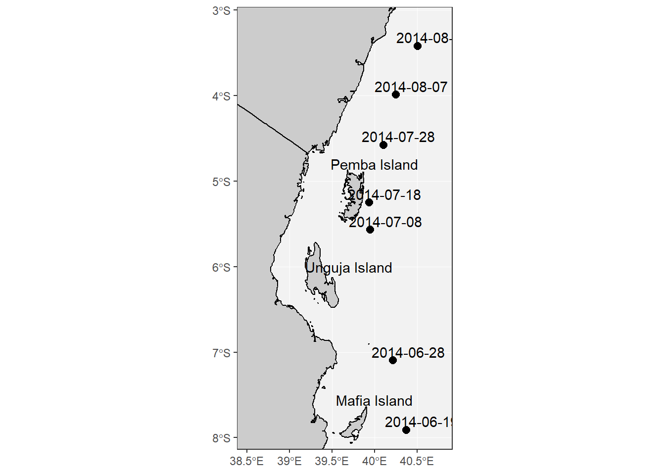
Figure 1: Map of the East African Coast showing the location of the Argo float profiles and the date the records were measured
Figure 2 show the vertical section of temperature as function of depth(to the maximum of 400 m) along the East African Coastal Current measured with Argo float with number 1901124 deployed by the CSIRO. This float crossed the East African coastal water between July 19 to August 17, 2014 and made seven profiles on Tanzania and Kenya waters. Looking Figure 2, although our eyes can clearly see the dermacation that separates the warm top water and bottom colder water, but it is hard to pinpoint the depth where the surface warm mixed layer end. Therefore, we must compute the MLD of these profiles using the temperature
## order the section and plot it
eacc.section = eacc.section %>%
  sectionSort(by = "latitude")
## plot the eacc section
eacc.section %>%
  plot(ztype = "image", ylim = c(400,20), xtype = "latitude", which = "temperature")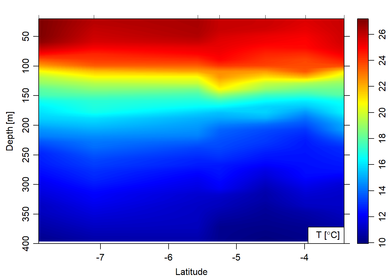
Figure 2: Hydrographic section of temperature and salinity
Estimate the MLD
To determine the MLD, we apply the method by Boyer Montégut et al. (2004), where successively deeper data points in each of the Argo profile potential temperature were examined until one is found with a potential temperature value differing from the value at the 10 m reference depth by more than the threshold value (\(\delta\)T)of \(\pm\) 0.5 oC. Using this approach, the MLD is then computed using a mathematic algorithm shown in the chunk below. In summary, the first line of the code preallocate the list file that will store the mld value for each profile. The For loop in the third line does the process of determing the mld. Notice that there is a nested loop that process the MLD. The first chunk prepare the data and the second loop is the main one that process the MLD
Figure 3 reveal that the MLD is not the same along the East African Coastal Current (EACC). The four profile off the coastal water of Tanzania have MLD range between 60 and 65 meters (Figure 3 top layer) and the deepest MLD was found further north off the Kenyan coast (Figure 3bottom right)
stations = eacc.section[["station"]]

mld.temp = list()

par(mfrow = c(2,4))

for (i in 1:length(stations)){
  # readline(prompt = "ENTER")
  ctd = stations[[i]]
  ctd = ctd %>% subset(pressure > 10)


      temperature = ctd[["temperature"]]
      pressure = ctd[["pressure"]]

    for (criterion in 0.5){
      inMLD =  abs(temperature[1] - temperature) < criterion
      MLDindex = which.min(inMLD)
      MLDpressure = pressure[MLDindex]

        ctd %>% plotProfile(xtype = "temperature", ylim = c(150,20))
        abline(h = pressure[MLDindex], lwd = 2, lty = "dashed")


        mld.temp[i] = MLDpressure

    }
}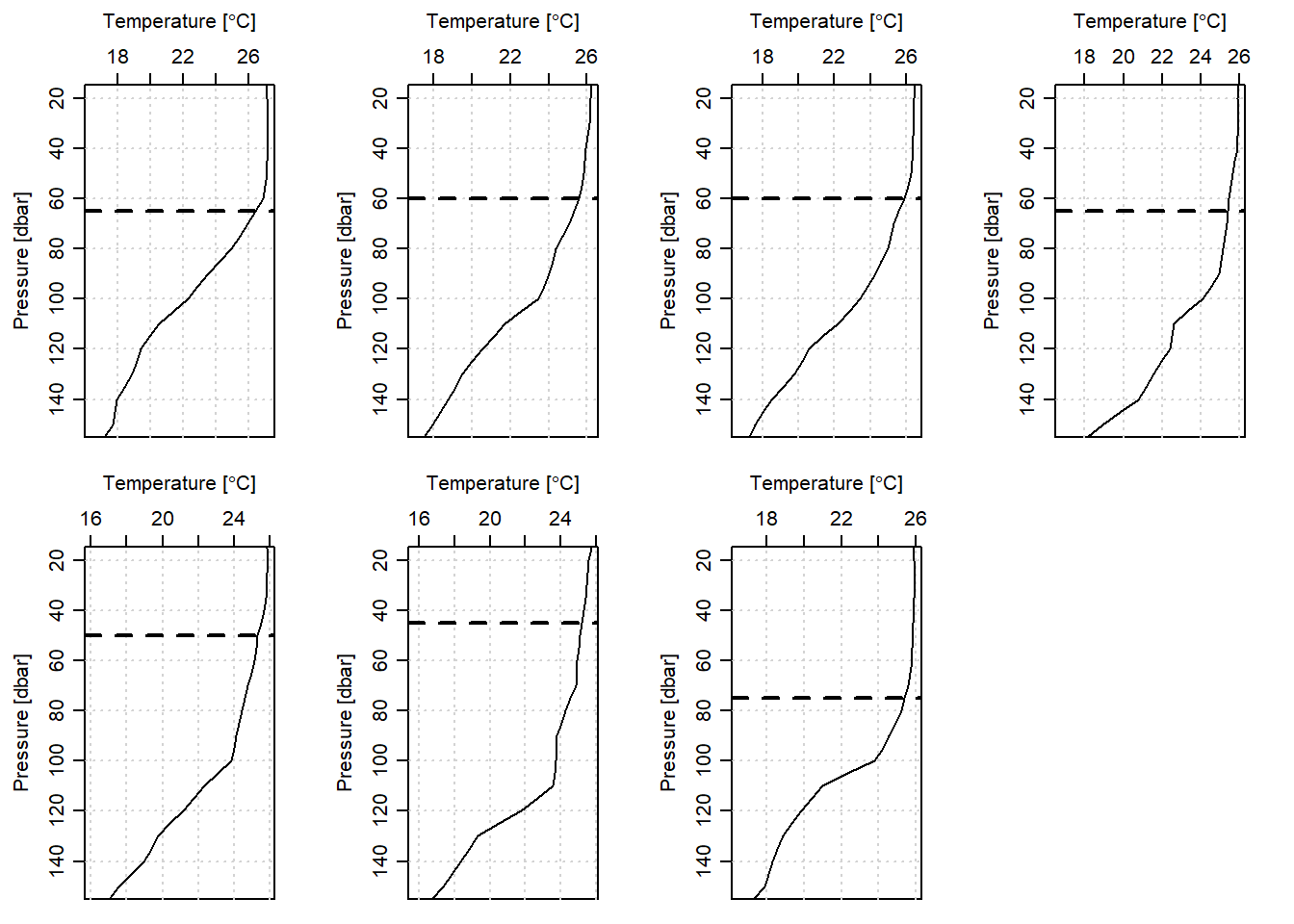
Figure 3: Mixed Layer Depth (MLD) for the seven profiles along the East African Coastal Current
Because the object mld.tempis in list form, It was converted into a data frame and then stitch it with the data frame created previous—containing the time, lon, and latitude of the profiles along the EACC. The following code chunk illustrates the process
mld.temp = mld.temp %>%
  as.data.frame() %>% t() %>%
  as.data.frame()%>%
  rename(mld = V1)

eacc.mld = eacc.extract.tb %>% bind_cols(mld.temp)
Table 1 reveal that during the southeast monsoon season (June to September), the water along the East African Coastal Current experience a shallow mixed layer depth of about 60 m.
| Date | Longitude | Latitude | MLD |
|---|---|---|---|
| 2014-06-19 | 40.372 | -7.909 | 65 |
| 2014-06-28 | 40.219 | -7.096 | 60 |
| 2014-07-08 | 39.951 | -5.570 | 60 |
| 2014-07-18 | 39.940 | -5.250 | 65 |
| 2014-07-28 | 40.103 | -4.577 | 50 |
| 2014-08-07 | 40.251 | -3.989 | 45 |
| 2014-08-17 | 40.506 | -3.419 | 75 |
Reference
Boyer Montégut, Clément de, Gurvan Madec, Albert S Fischer, Alban Lazar, and Daniele Iudicone. 2004. “Mixed Layer Depth over the Global Ocean: An Examination of Profile Data and a Profile-Based Climatology.” Journal of Geophysical Research: Oceans 109 (C12). Wiley Online Library.
Costoya, Xurxo, Maite deCastro, Moncho Gómez-Gesteira, and Fran Santos. 2014. “Mixed Layer Depth Trends in the Bay of Biscay over the Period 1975–2010.” Journal Article. PLOS ONE 9 (6): e99321. doi:10.1371/journal.pone.0099321.
Kelley, Dan, and Clark Richards. 2018. Oce: Analysis of Oceanographic Data. https://CRAN.R-project.org/package=oce.
R Core Team. 2018. R: A Language and Environment for Statistical Computing. Vienna, Austria: R Foundation for Statistical Computing. https://www.R-project.org/.