Determine dynamic height and geostrophic velocity along the East African Coastal Current from Argo floats

Introduction

I have been working with argo floats data and wrote two post that illustrate how to detect the mixed layer depth with criterion and derivative approaches. In this post, I change the focus. Rather than talking about the mixed layer depth detection, I will illustrate how to calculate the dynamic height and geostrophic velocity from same dataset—Argo float. I use R programming language as an environment for the required routine to calculate the dynamic height and geostrophic current (R Core Team 2018). To accomplish this process I need several packages. You can achieve the process just by relying on the base R. but, Kelley and Richards (2018) developed oce package that makes R programming languages (R Core Team 2018) capable of handling and analysing wide variety of oceanographical data. As usual, I need to load the necessary packages into the workspace required for importing (Kelley and Richards 2018; Pebesma 2018), processing argo dataset (Kelley 2018; Wickham and Henry 2018), mapping (Pebesma 2018) and displaying the outputs (Wickham 2017).

require(tidyverse)
require(oce)
require(ocedata)
require(sf)
require(lubridate)

Read Argo file with oce package

In this post I used freely available Argo floats profile of salinity and temperature that crossed the coastal water of Tanzania and Kenya. Argo data were obtained as the actual Argo NetCDF files from the Argo Data website. Argo recommends the delayed mode for oceanographic application because the profiles of salinity and temperature has been adjusted with high quality ship-based CTD and climatological data. Each Argo floats comes with four different files—the first file is profile, which contains all measured profiles; second file is the trajectory, which contains consecutive position information (longitude, latitude and time) of the float while the float is a surface sending data to satellite; the third file is metadata. It contains the float and sensor characteristics; and the fourth file is technical one that store the information of the instrument like battery voltages and intensities.

Because there were 51 NetCDF file of different float in the region, I first created a directory file that list the names and path of each dataset.

argo.float = argo[39]%>% 
  read.argo()%>% 
  handleFlags() %>% 
  argoGrid(p = seq(5,400,5))

Once the the argo float dataset has been cleaned, we can extract important information like the longitude, latitude and time the profile was recorded

time = argo.float[["time"]]
lon = argo.float[["longitude"]]
lat = argo.float[["latitude"]]

make a section

Because the profiles are in list format, we can convert them directly into section with with as.section() function

argo.section = argo.float%>%  
  as.section()

subset the EACC from the dataset

The section provide a nifty way to subset only the profile we are interested. I did a simple exploration and found that the profile number 206 to 212 cover well the EACC. Therefore, we only pick these profile and drop the rest from the dataset. Because I also need to know the time of each profile, I selected the time and location information using the index method and make a data frame of these information. Figure 1 show the location of the profile and the time in which the measurement were done and figure 2 hydrographic section of these station to 200 meter deep

## make a section from list of argo profile
eacc.section = argo.section %>% subset(stationId  >= 206 & stationId <= 212)

## obtain the time and spatial information corresponding to each profile
time.eacc = time[206:212] %>% as.Date()
lon.eacc = lon[206:212]
lat.eacc = lat[206:212]

## create a table from the time, lon and lat variable extracted above
eacc.extract.tb = data.frame(time.eacc, lon.eacc, lat.eacc) %>% 
  rename(time = 1, lon = 2, lat = 3)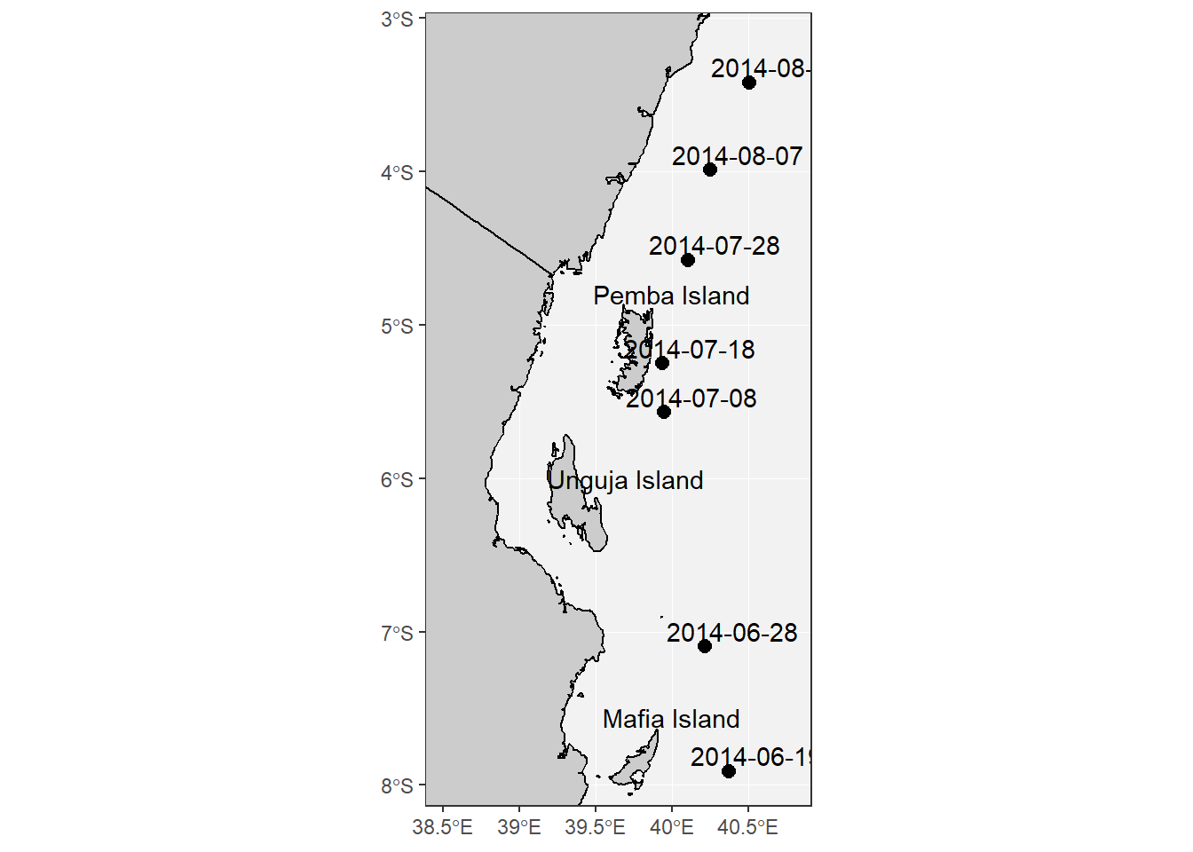

Figure 1: Map of the East African Coast showing the location of the Argo float profiles and the date the records were measured

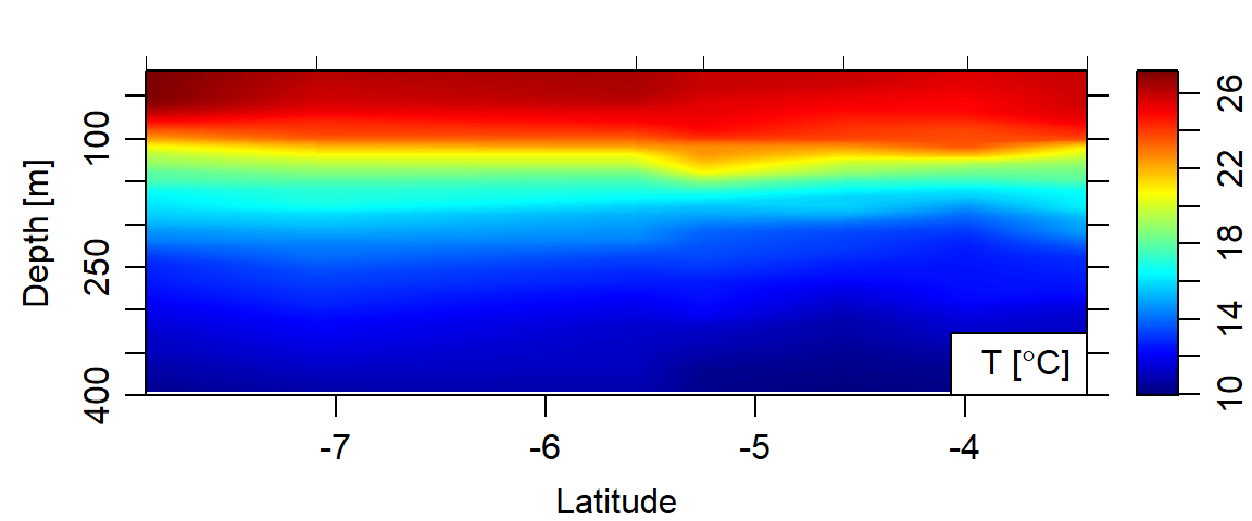
Figure 2: Hydrographic section of temperature

Compute the Dynamic height

From the hydrographic section of the East African Coastal current (EACC) obtained from the Argo float, the dynamic height for each station was computed using the swDynamicHeight() function. The chunk below shows all the three main line of code required for the process. The output is a list file contains distance and dynamic height for each station along the section.

## calculate  and plot dynamic height
eacc.dh = eacc.section %>% 
  sectionSort(by = "latitude") %>%
  swDynamicHeight() 

# plot(eacc.dh$distance, eacc.dh$height, type = "l", 
#ylab = "Dynamic Height (m)", xlab = "Distance (km)")

The computed dynamic height along the East African coastal current are shown in figure 3. The figure reveal that the dynamic height increased from latitude 8^oS to 7^oS and decreased slightly to latitude 4^oS. This findings suggest that the EACC flows along the decreasing dynamic height during the southeast season.

eacc.dh.df = eacc.dh %>% as.data.frame()
## get latitude from the section for labelling the x-axis
lat = eacc.section@metadata$latitude
## add latitude colum
eacc.dh.df = data.frame(lat,eacc.dh.df)

ggplot(data = eacc.dh.df, aes(x = lat, y = height)) + 
  geom_line(size = 1.2, col = "red") +
  theme(panel.background = element_rect(colour = "black"),
        axis.text = element_text(size = 11),
        axis.title = element_text(size = 12),
        panel.grid.minor = element_blank())+
  labs(y = "Dynamic Height (m)", x = "Latitude")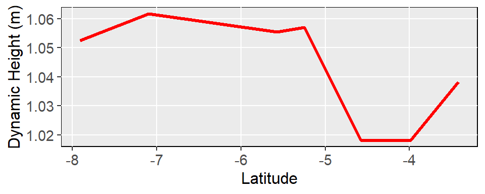

Figure 3: Dynamic Height along the EACC derived from Argo float

Compute Geostrophic Height

Once the dynamic height along the EACC current was determined, we can proceed with the computation of the geostrophic velocity. The code for the process is shown in the chunk below. In summary, the first thing is to determine the coriolis force (\(f\)) and acceleration due to gravity (\(g\)). The coriolis force (\(f\)) and acceleration due to gravity (\(g\)) as a function of latitude were computed from latitude using method described by Gill (1982) and Groten (1997). Then the geostrophic current velocity (\(gv\)) was computed using the equation (1).

\[ \begin{equation} gv = \frac{\frac{\Delta \: DH_i}{\Delta \:D_i} \times g}{ f \times 1000} \tag{1} \end{equation} \]

Where the \(i\) subscript refer to the individual latitude, \(\Delta dh\) = change in dynamic height; \(\Delta distance\) = change in distane; \(g\) = accelation due to gravity; \(f\) = coriolis force. In carrying out this calculation, the change in the dynamic height along the latitude was divided by the change in distance. Multiplying by the accelation due to gravity (\(g\)) and divide with coriolis force (\(f\)) and 1000 to obtain the geostrophic velocity at each latitude shown in figure 4.

## get latitude value along the EACC from the section object
lat = eacc.section@metadata$latitude%>%round(2)
## 
f = coriolis(lat) ## derive coriolis force
g = gravity(lat) ## derive acceleration due to gravity

## then cacluate and plot the geostrophic velocity
gv = diff(eacc.dh$height) / diff(eacc.dh$distance) * g / f / 1000

## make a data frame for plotting with ggplot2
eacc.dh.gv.df = data.frame(lat,gv)

## plot(eac.dh$distance, gv, type = "l", ylab = "Velocity (m/s)", xlab = "Distance (km)")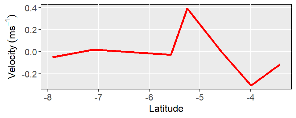

Figure 4: Geostrophic velocity derived from Argo float along the EACC