A map projection is a way to flatten a globe’s surface into a plane in order to make a map. This requires a systematic transformation of the latitudes and longitudes of locations from the surface of the globe into locations on a plane.[1] All projections of a sphere on a plane necessarily distort the surface in some way and to some extent. Depending on the purpose of the map, some distortions are acceptable and others are not; therefore, different map projections exist in order to preserve some properties of the sphere-like body at the expense of other properties. Every distinct map projection distorts in a distinct way, by definition.
Projections are grouped according to properties of the model they preserve. Some of the more common categories are;
- cylindrical (e.g. Mercator),
- conic (e.g. Albers), and
- plane (e.g. stereographic)
The three developable surfaces (plane, cylinder, cone) provide useful models for understanding, describing, and developing map projections. However, these models are limited in two fundamental ways. For one thing, most world projections in use do not fall into any of those categories. For another thing, even most projections that do fall into those categories are not naturally attainable through physical projection.
In this post I will take you through the projection that are commonly and widely used to map features on the earth surface. First we need to load the sf package that support for simple features—a standardized way to encode spatial vector—point, lines and polygons (Pebesma 2018). The other package that we need is the tidyverse, a set of packages that we use for mapping and data manipulation (Wickham 2017). Let’s load the package into our session
require(sf)
require(tidyverse)
I assume that you are familiar with spatial data construction and that is not the focus of this post. You can use any spatial data that you know, but for this post I will use the world spatial data bundled in the spData package (Bivand, Nowosad, and Lovelace 2020). The dataset is the simple feature and contains a records of 177 countries with 11 variables. We can simply load the data set as the highlighted in the chunk below.
dunia = spData::world %>%
  st_as_sf()
EPSG code
The EPSG codes are assigned to Geographical Coordinate System (GCS), coordinate transformation and their components. Therefore, instead of remembering all the details for a particular coordinate system, you simply parse the epsg code and the mapping software recognize and respond to that particular projections and its transformations. For more details please visit projection link. Therefore, the maps that follows below are generated with different projections
ggplot() +
  ggspatial::layer_spatial(data = dunia)+
  coord_sf(crs = 4326) +
  ggtitle("WGS 84 - WGS84 - World Geodetic System 1984, used in GPS")+
  cowplot::theme_minimal_grid()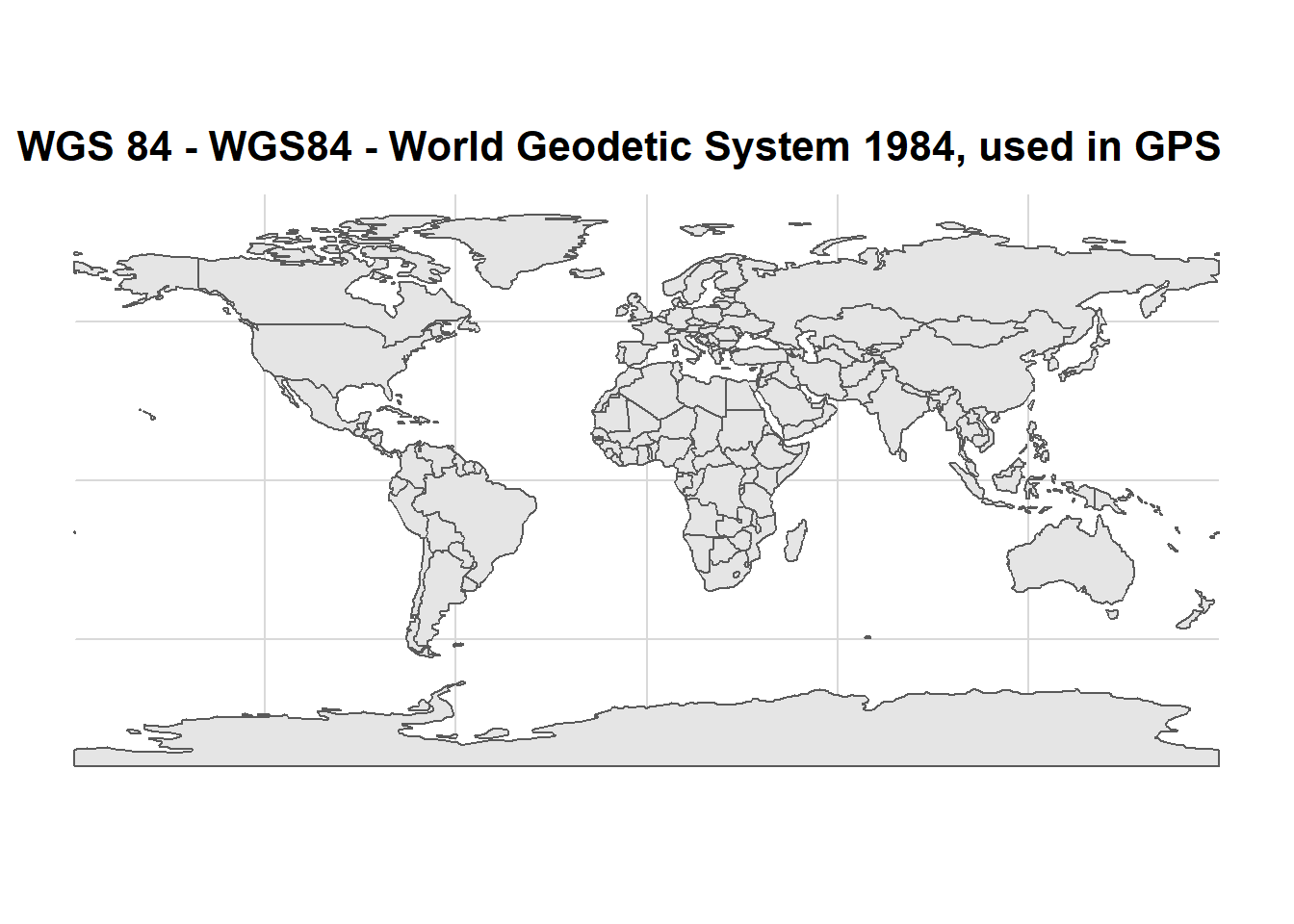
ggplot() +
  ggspatial::layer_spatial(data = dunia)+
  coord_sf(crs = 3395) +
  ggtitle("WGS 84 / World Mercator")+
  cowplot::theme_minimal_grid()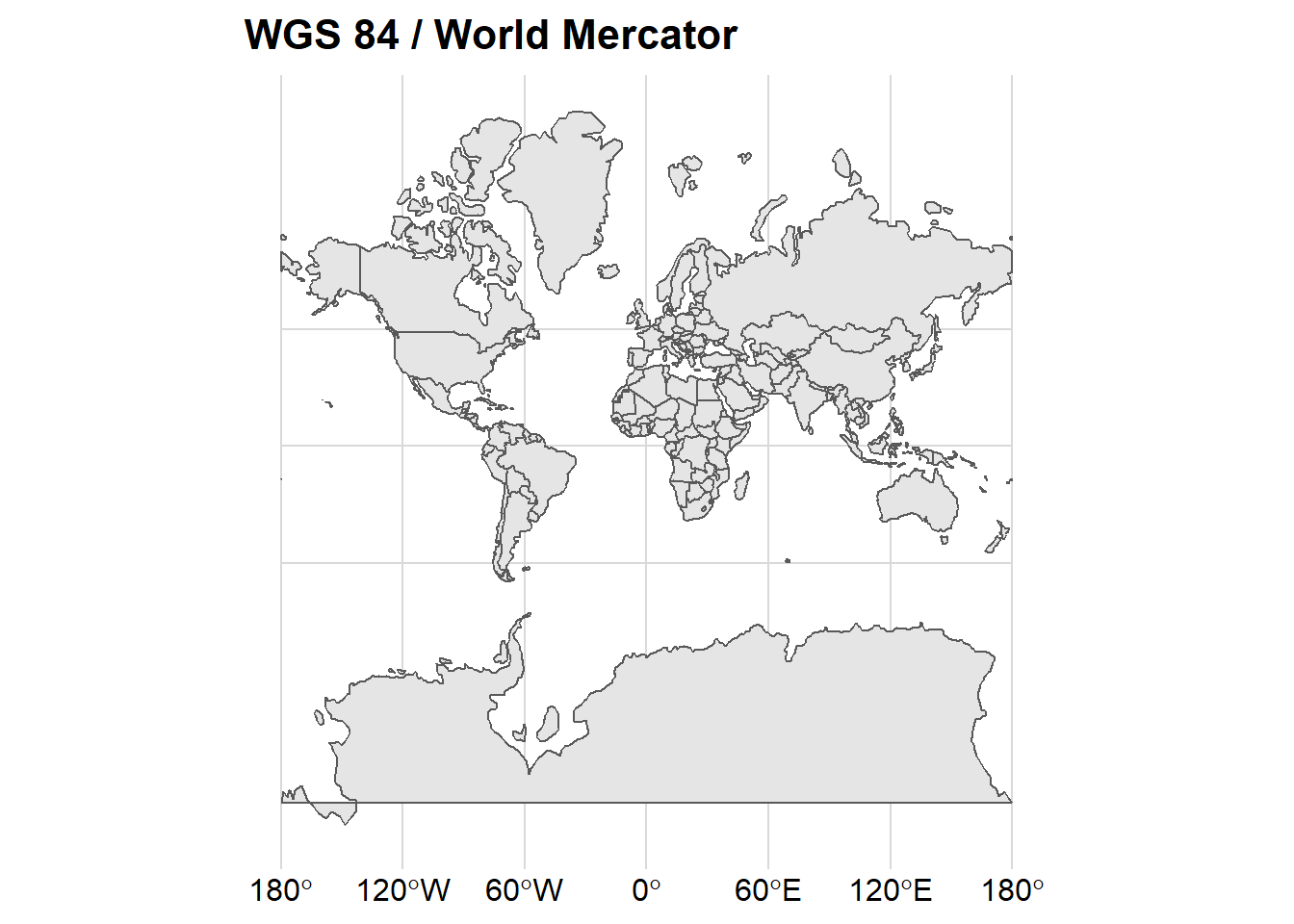
ggplot() +
  ggspatial::layer_spatial(data = dunia)+
  coord_sf(crs = 4087) +
  ggtitle("WGS 84 / World Equidistant Cylindrical")+
  cowplot::theme_minimal_grid()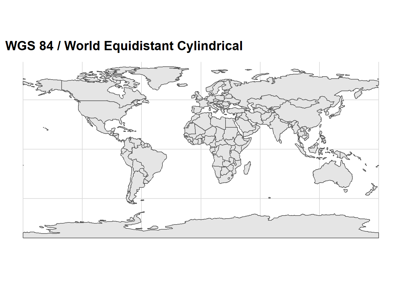
ggplot() +
  ggspatial::layer_spatial(data = dunia)+
  coord_sf(crs = 4088) +
  ggtitle("World Equidistant Cylindrical (Sphere)")+
  cowplot::theme_minimal_grid()
ggplot() +
  ggspatial::layer_spatial(data = dunia)+
  coord_sf(crs = 54030) +
  ggtitle("World Robinson")+
  cowplot::theme_minimal_grid() +
  scale_fill_viridis_c()
ggplot() +
  ggspatial::layer_spatial(data = dunia)+
  coord_sf(crs = 54024) +
  ggtitle("World Bonne")+
  cowplot::theme_minimal_grid()+
  cowplot::theme_minimal_grid()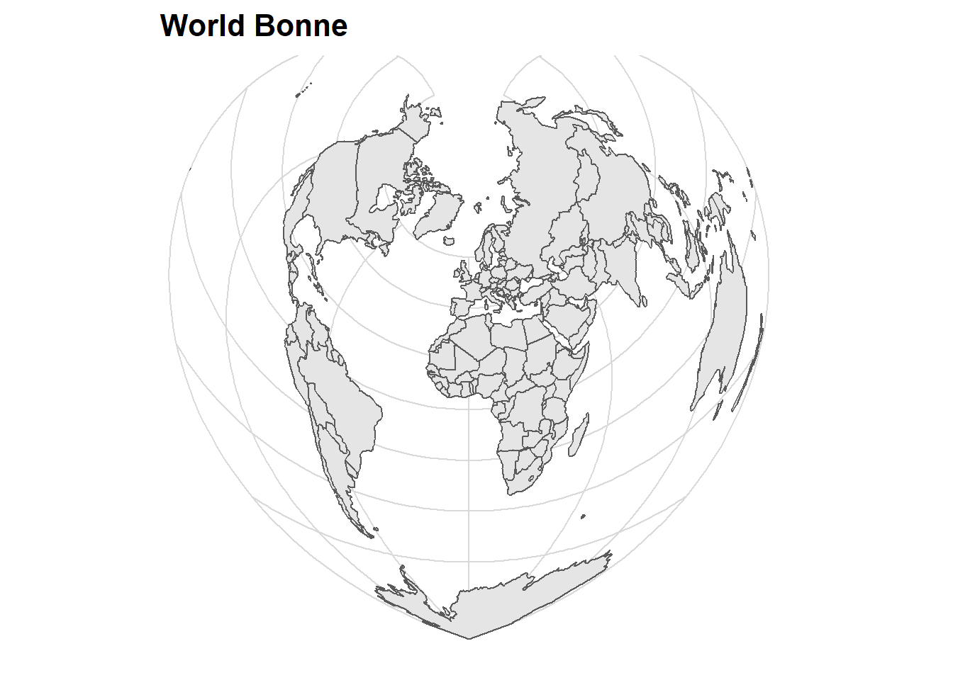
ggplot() +
  ggspatial::layer_spatial(data = dunia)+
  coord_sf(crs = 54021) +
  ggtitle("World Polyconic")+
  cowplot::theme_minimal_grid()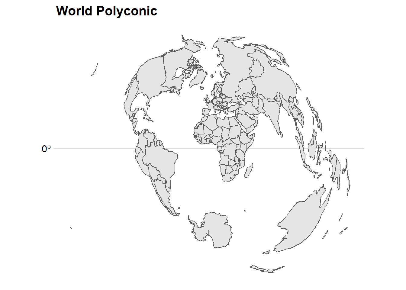
nc = ncdf4::nc_open("e:/GIS/ROADMAP/LAYERS DATA/GLOBAL LAYERS/coads/airtemp/airtemp_jan_global_coads_nvods.nc")
ait = ncdf4::ncvar_get(nc, "AIRT")
lon = ncdf4::ncvar_get(nc, "COADSXN100_80")
lat = ncdf4::ncvar_get(nc, "COADSY")


air.data = expand.grid(lon,lat)  %>%
  bind_cols(
    ait %>% expand.grid()
    ) %>%
  rename(lon = 1, lat = 2, air.temperature = 3)

air.raster = raster::raster("e:/GIS/ROADMAP/LAYERS DATA/GLOBAL LAYERS/coads/airtemp/airtemp_jan_global_coads_nvods.nc")

air.tb = air.raster %>%
  raster::as.data.frame(xy = TRUE) %>%
  rename(lon = 1, lat = 2, air.temperature = 3)
ggplot() +
# geom_raster(data = air.data, aes(x = lon, y = lat, fill = air.temperature))+
# geom_raster(data = air.tb, aes(x = lon, y = lat, fill = air.temperature))+
# ggspatial::layer_spatial(data = dunia)+
geom_sf(data = dunia)+
coord_sf(crs = 54009) +
ggtitle("World Mollweide")+
cowplot::theme_minimal_grid()+
scale_fill_gradientn(colours = oce::oce.colors9A(120), na.value = "white")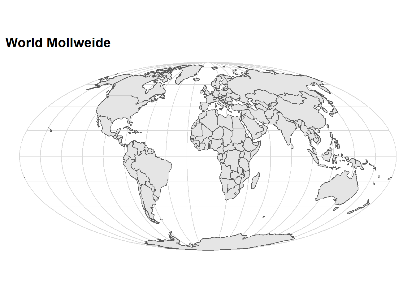
ggplot() +
  ggspatial::layer_spatial(data = dunia)+
  coord_sf(crs = 54032) +
  ggtitle("World Azimuthal Equidistant")+
  cowplot::theme_minimal_grid()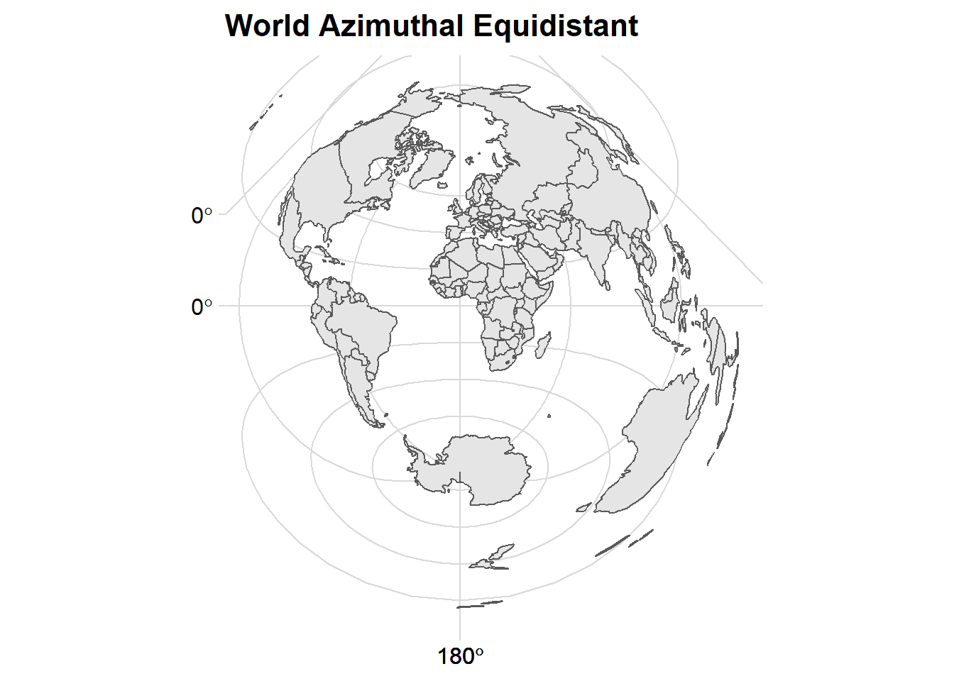
ggplot() +
  ggspatial::layer_spatial(data = dunia)+
  coord_sf(crs = 54016) +
  ggtitle("World Gall Stereographic")+
  cowplot::theme_minimal_grid()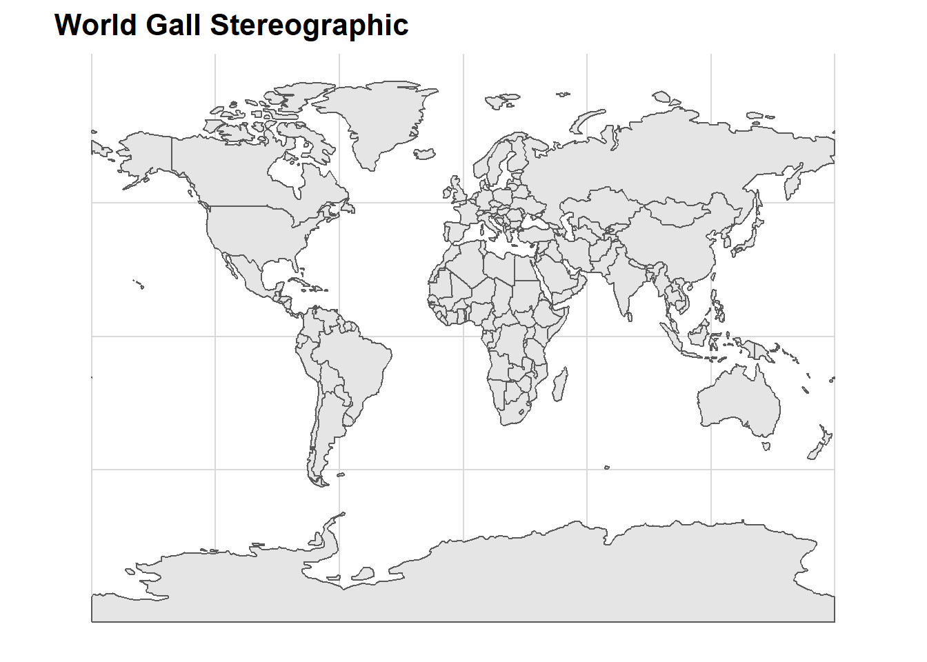
ggplot() +
  ggspatial::layer_spatial(data = dunia)+
  coord_sf(crs = 54013) +
  ggtitle("World Eckert III")+
  cowplot::theme_minimal_grid()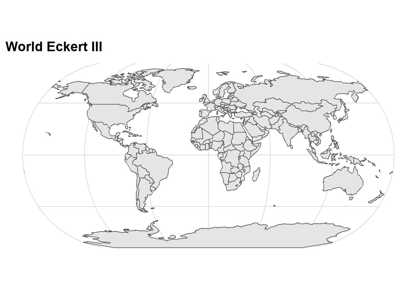
ggplot() +
  ggspatial::layer_spatial(data = dunia)+
  coord_sf(crs = 54012) +
  ggtitle("World Eckert IV")+
  cowplot::theme_minimal_grid()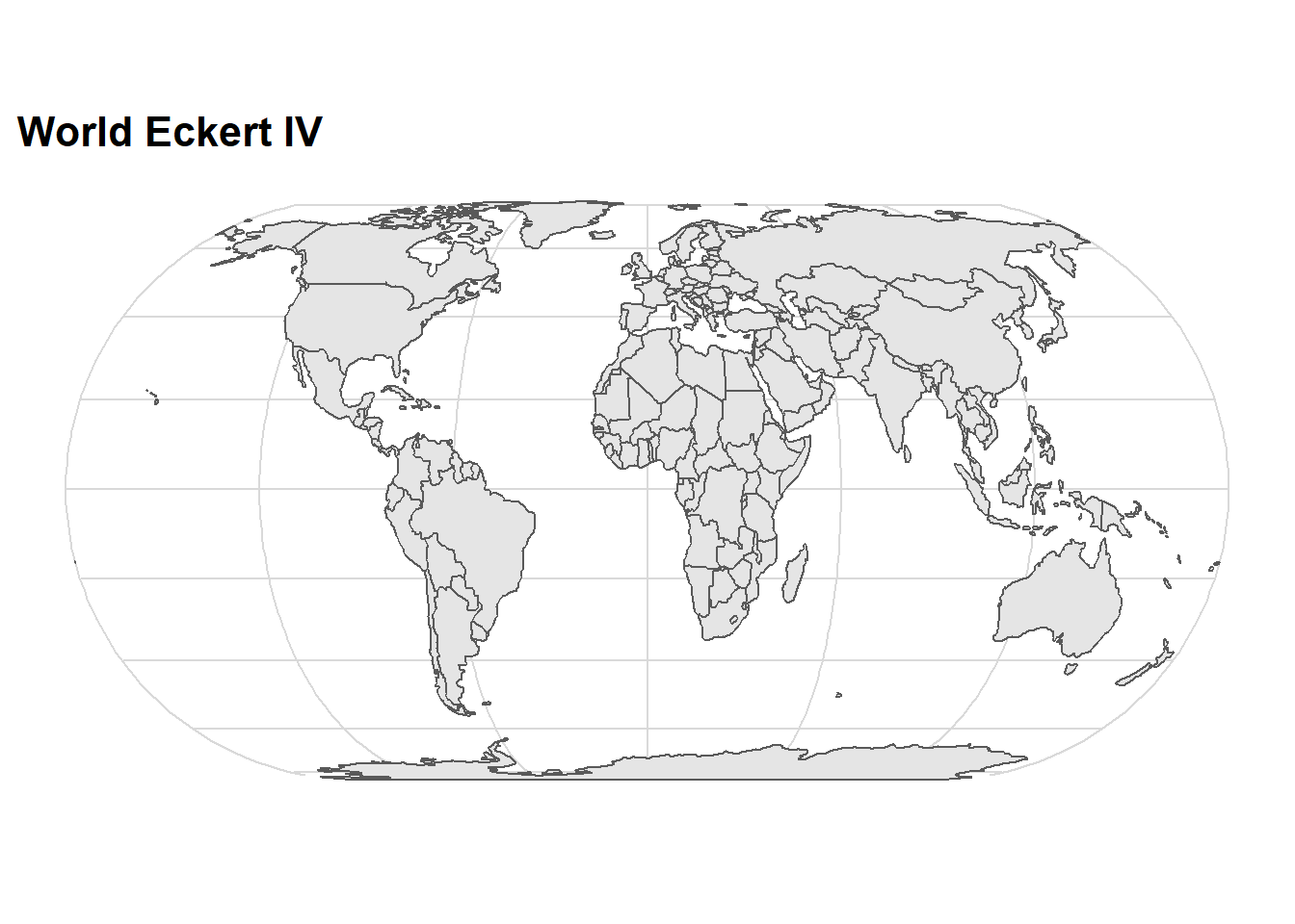
ggplot() +
  ggspatial::layer_spatial(data = dunia)+
  coord_sf(crs = 54010) +
  ggtitle("World Eckert VI")+
  cowplot::theme_minimal_grid()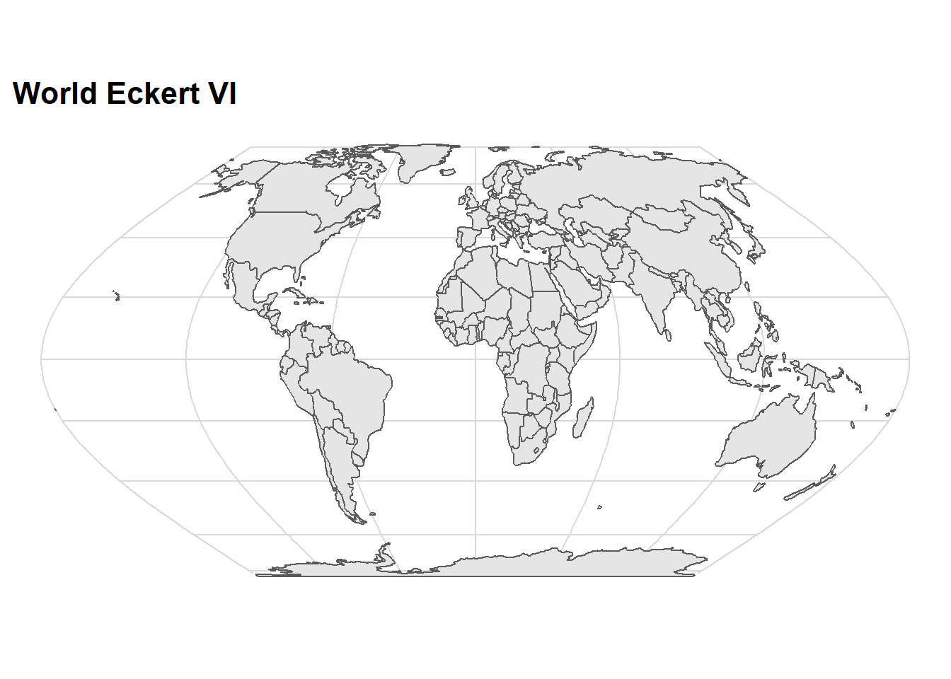
ggplot() +
  ggspatial::layer_spatial(data = dunia)+
  coord_sf(crs = 54003) +
  ggtitle("World Miller Cylindrical")+
  cowplot::theme_minimal_grid()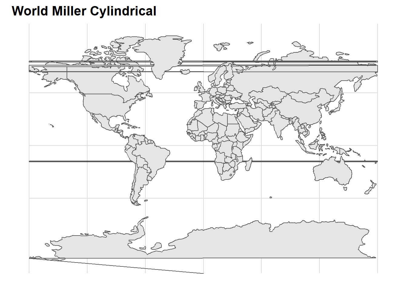
ggplot() +
  ggspatial::layer_spatial(data = dunia)+
  coord_sf(crs = 54002) +
  ggtitle("World Equidistant Cylindrical")+
  cowplot::theme_minimal_grid()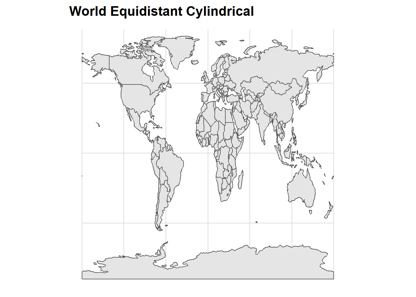
ggplot() +
  ggspatial::layer_spatial(data = dunia)+
  coord_sf(crs = 54001) +
  ggtitle("World Plate Carree")+
  cowplot::theme_minimal_grid()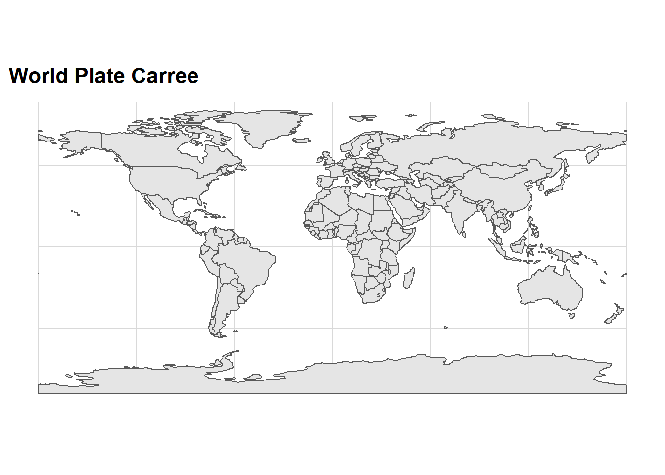
ggplot() +
  ggspatial::layer_spatial(data = dunia)+
  coord_sf(crs = 54031) +
  ggtitle("World Two Point Equidistant")+
  cowplot::theme_minimal_grid()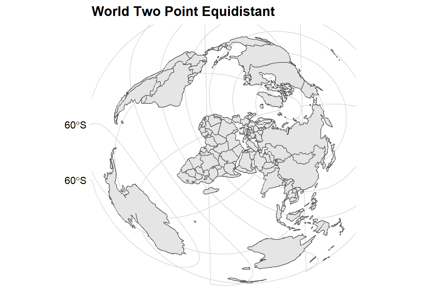
ggplot() +
  ggspatial::layer_spatial(data = dunia)+
  coord_sf(crs = 4088) +
  ggtitle("World Equidistant Cylindrical (Sphere)")+
  cowplot::theme_minimal_grid()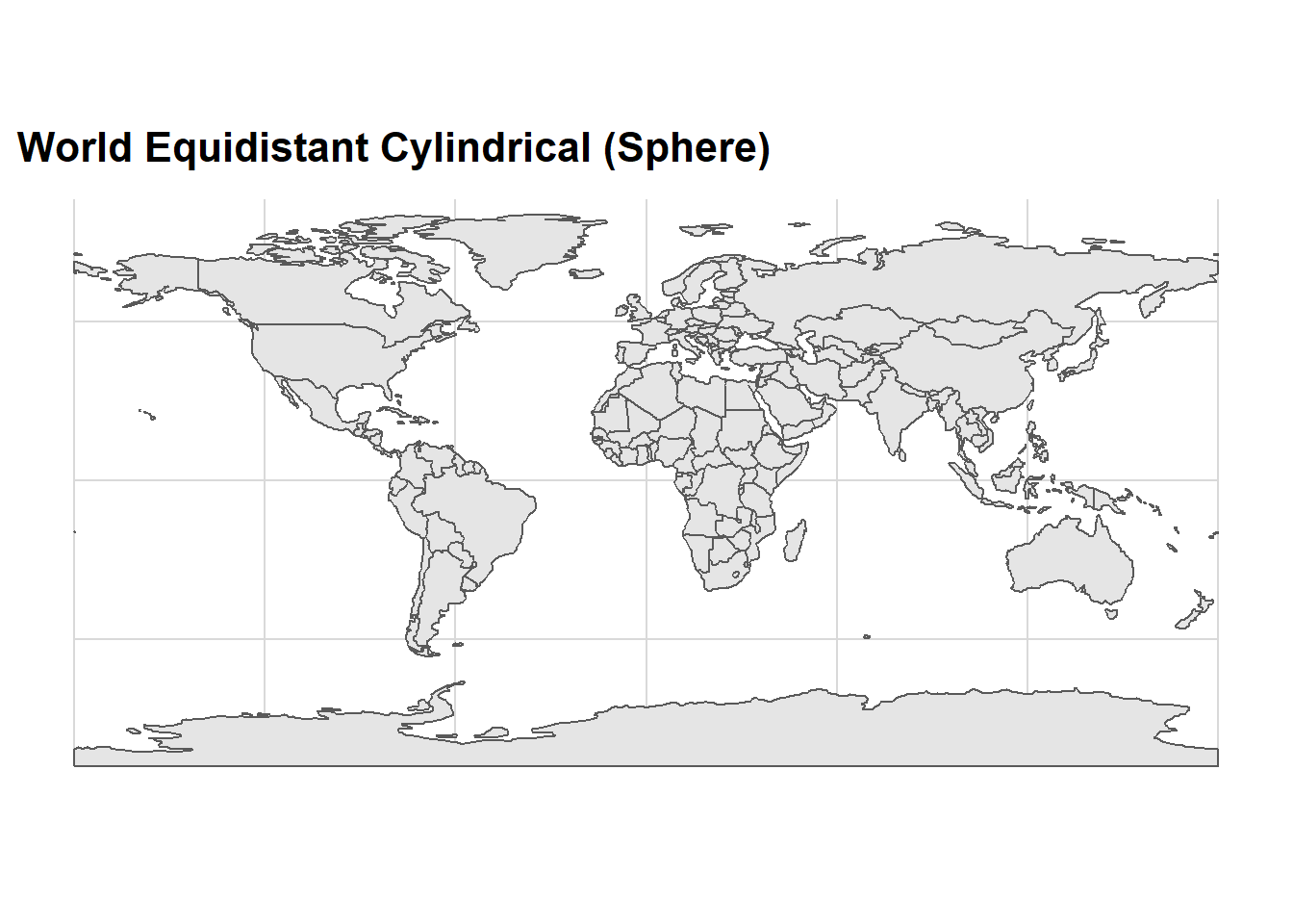
References
Bivand, Roger, Jakub Nowosad, and Robin Lovelace. 2020. SpData: Datasets for Spatial Analysis. https://CRAN.R-project.org/package=spData.
Pebesma, Edzer. 2018. Sf: Simple Features for R. https://CRAN.R-project.org/package=sf.
Wickham, Hadley. 2017. Tidyverse: Easily Install and Load the ’Tidyverse’. https://CRAN.R-project.org/package=tidyverse.